多视图几何(八)
Chapter8 Direct Approaches to Visual SLAM
8.1 Classical Approaches to Multiple View Reconstruction
In the past chapters we have studied classical approaches to multiple view reconstruction. These methods tackle the problem of structure and motion estimation (or visual SLAM) in several steps:
- A set of
feature pointsis extracted from the images -ideally points points such ascornerswhich can be reliably identified in subsequent images as well. - One determines a
correspondence of these points across the various images. This can be done either through local tracking (using optical flow approaches) or by random sampling of possible partners based on a feature descriptor (SIFT, SURF, etc.) associated with each point, - The
camera motion is estimatedbased on a set of corresponding points. In many approaches this is done by a series of algorithms such as the8-point algorithmor the5-point algorithmfollowed bybundle adjustment. - For a given camera motion one can then compute a
dense reconstructionusing photometric stereo approaches.
8.2 Shortcomings of Classical Approaches
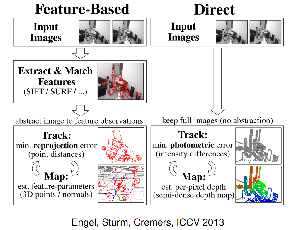
Such classical approaches are indirect in the sense that they do not compute structure and motion directly from the images but rather from a sparse set of precomputed feature points. Despite a number of successes, they have several drawbacks:
- From the point of view of statistical inference, they are
suboptimal: In the selection of feature points much potentially valuable information contained in the colors of each images is discarded. - They invariably
lack robustness: Error in the point correspondence may have devastating effects on the estimated camera motion. Since one often selects very few point pairs only (8 points for the 8-point algorithm, 5 points for the 5-point algorithm), any incorrect correspondence will lead to an incorrect motion estimate. - They do not address the
highly coupled problems of motion estimation and dense structure estimation. They merely do so for a sparse set of points. As a consequence, improvements in the estimated dense geometry will not be used to improve the camera motion estimates.
8.3 Toward Direct Approaches to Multiview Reconstruction
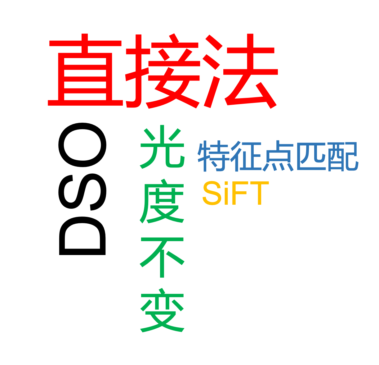
In the last few years, researchers have been promoting direct approaches to multi-view reconstruction. Rather than extracting a sparse set of feature points to determine the camera motion, direct methods aim at estimating camera motion and dense or semi-dense scene geometry directly from the input images. This has several advantages:
- Direct methods tend to be
more robustto noise and other nuisances because theyexploit all variable input information. - Direct methods provide a
semi-dense geometric reconstructionof the scene which goes well beyond the sparse point cloud generated by the 8-point algorithm or bundle adjustment. Despending on the application, a separate dense reconstruction step may no longer be necessary. - Direct methods are
typically fasterbecause the feature-point extraction and correspondence finding is omitted: They can provide fairly accurate camera motion and scene structure in real-time on a CPU.
8.4 Feature-Based versus Direct Methods
8.5 Direct Methods for Multi-view Reconstruction
In the following, we will briefly review several recent works on direct methods for multiple-view reconstruction:
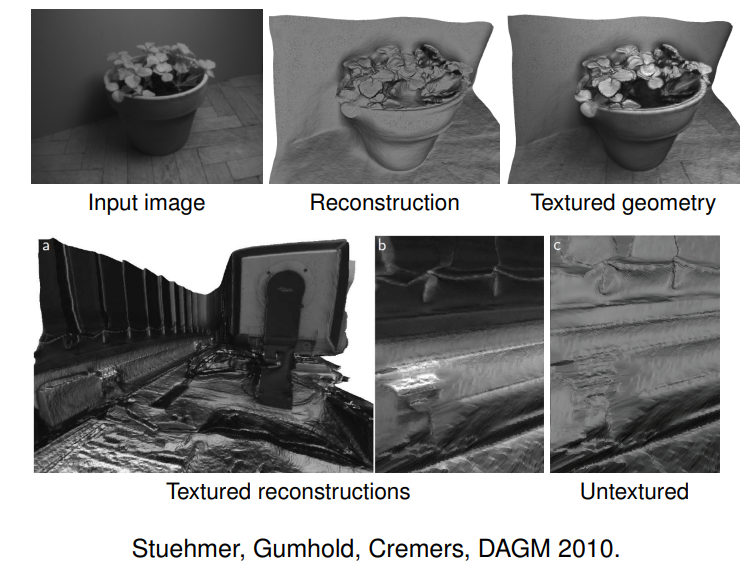
- the method of
Stühmer, Gumhold, Cremers, DAGM 2010computes dense geometry from a handheld camera in real-time. - the methods of
Steinbrücker, Sturm, Cremers, 2011 and Kerl, Sturm, Cremers, 2013directly compute the camera motion of an RGB-D camera. - the method of
Newcombe, Lovegrove, Davison, ICCV 2011directly determines dense geometry and camera motion from the images. - the method of
Engel, Sturm, Cremers, ICCV 2013andEngel, Schöps Cremers, ECCV 2014directly computes camera motion and semi-dense geometry for a handheld (monocular) camera. - the method of
Engel, Koltun, Cremers, PAMI 2018directly estimates highly accurate camera motion and sparse geometry.
8.6 Realtime Dense Geometry from a Handheld Cameara
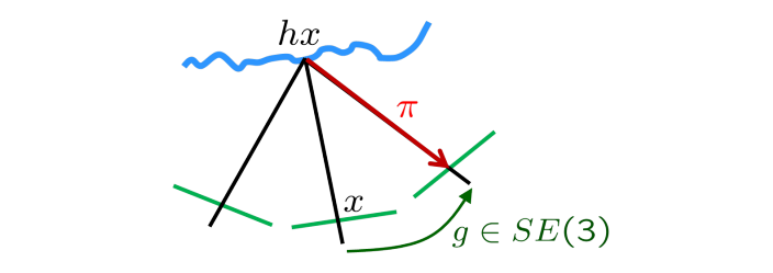
Let $g_i \in SE(3)$ be the rigid body motion from the first camera to the $i$-th camera, and let $I_i: \Omega \rightarrow \mathbb{R}$ be the $i$-th image. A dense depth map $\textcolor{green}{h: \Omega\rightarrow \mathbb{R}}$ can be computed by solving the opyimization problem:
$$
\min_{h} \sum_{i=2}^n \int_{\Omega} |I_1(\textbf{x}) -I_i(\pi g_i(h\textbf{x}))|d\textbf{x} + \lambda \int_{\Omega} |\bigtriangledown h|d\textbf{x},
$$
where $\textbf{x}$ is represented in homogeneous coordinates and $h\textbf{x}$ is the corresponding 3D point.
Like in optical flow estimation, the unknown depth map should be such that for all pixels $\textbf{x}\in \Omega$, the transformation into the other images $I_i$ should give rise to the same color as in the reference image $I_1$.
This cost function can be minimized at framerate by coarse-to-fine linearlization solved in parallel on a GPU.
8.7 Dense RGB-D Tracking
The approach of Stühmer et al. (2010) relies on a sparse feature-point based camera tracker (PTAM) and computes dense geometry directly on the images. Steinbrücker, Sturm, Cremers (2011) propose a complementary approach to directly compute the camera motion from RGB-D images. The idea is to compute the rigid body motion $g_\xi$ which optimally alogns two subsequent color images $I_1$ and $I_2$:
$$
\min_{\xi \in \mathfrak{se}(3)}\int_{\Omega} |I_1(\mathrm{x}) - I_2(\pi g_\xi (hx))|^2 d\mathrm{x}
$$
The above non-convex problem can be approximated as a convex problem by linearizing the residuum around an initial guess $\xi_0$:(在$\xi_0$处进行一阶泰勒展开 )
$$
E(\xi) = \int_{\Omega}|I_1(\textbf{x}) - I_2(\pi g_{\xi_0}(h\textbf{x}))-\bigtriangledown I_2^\top(\frac{d\textcolor{red}{\pi}}{d\textcolor{green}{g_\xi}})(\frac{d\textcolor{green}{g_\xi}}{d\xi})\xi|^2 d\textbf{x}
$$
This is a convex quadratic cost function which gives rise to a linear optimality condition:
$$
\frac{dE(\xi)}{d\xi} = A \xi + b = 0
$$
To account for larger motions of the camera, this problem is solved in a coarse-to-fine manner. The linearization of the residuum is identical with a Gauss-Newton approach. It corresponds to an approximation of the Hessian by a positive definite matrix.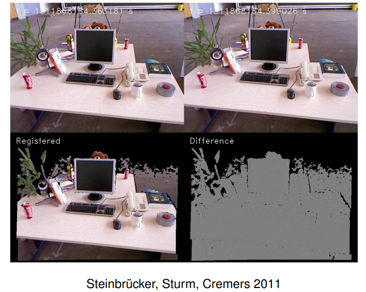
 wechat
 alipay