Chapter7 Bundle Adjustment & Nonlinear Optimization

7.1 Optimality in Noisy Real World Conditions

In the previous chapters we discussed linear approaches to solve the structure and motion problem. In particular, the 8-point algorithm provides closed-form solutions to estimate the camera parameters and the 3D structure, based on singular value decomposition. (SVD)

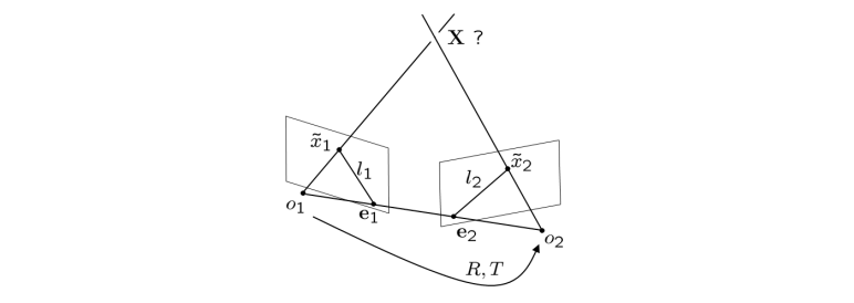
However, if we have noisy data $\tilde{\textbf{x}_1}, \tilde{\textbf{x}_2}$ (correspondence not exact or even incorrect), then we have no guarantee:

that $R$ and $T$ are as close as possible to the true solution.
that we will get a consistent reconstruction.

7.2 Statistical Approaches to Cope with Noise

The linear approaches are elegant because optimal solutions to respective problems can be computed in closed form.

However, they often fail when dealing with noisy and imprecise point locations. Since measurement noise is not explicitly considered or modeled, such spectral methods often provide suboptimal performence in noisy real-world conditions.

In order to take noise and statistical flucation into account, one can revert to a Bayesian formulation and determine the most likely camera transformation $R, T$ and ‘true’ 2D coordinates ${x}$ givens the measured coordinates $\tilde{\textbf{x}}$, by perfroming a maximum a posteriori estimate:

$$
\underset{\textbf{x}, R, T}{argmax} \mathcal{P}(\textbf{x}, R, T |\tilde{\textbf{x}}) = \underset{\textbf{x},R,T}{argmax} \mathcal{P}(\tilde{\textbf{x}}|\textbf{x},R,T)\mathcal{P}(\textbf{x}, R, T)
$$

(Note: 后验概率= 似然概率 * 先验概率)

This approach will however involve modeling probability densities $\mathcal{P}$ on the fairly complicated space $SO(3)\times \S^2$ of rotation and translation parameters, as $R\in SO(3)$ and $T\in \S^2$(3D translation with unit length).

7.3 Bundle Adjustment and Nonlinear Optimization

Under the assumption that the observed 2D point coordinates $\tilde{\textbf{x}}$ are corrupted by zero-mean Gaussian noise, maximum likelihood estimation leads to bundle adjustment:

$$
\textbf{E}(R, T, \textbf{X}_1, …, \textbf{X}_N)=\sum_{j=1}^N |\tilde{\textbf{x}_1}^j -\pi (\textbf{X}_j)|^2 + |\tilde{\textbf{x}_2}^j - \pi(R, T, \textbf{X}_j)|^2,
$$

where $\textcolor{green}{\pi(R,T,\textbf{X}_j)} = \textcolor{green}{(R\textbf{X}_j+ T)}$

It aims at minimizing the reprojection error between the observed 2D coordinates $\tilde{\textbf{x}_i}^j$ and the projected 3D coordinate $\textbf{X}_j (w.r.t camera 1)$. Here $\pi(R,T,\textbf{X}_j)$ denotes the perspective projection of $\textbf{X}_j$ after rotation and translation.

For the general case of m images, we get:

$$
\textbf{E}({R_i, T_i}_{i=1,…,m}, {\textbf{X}_j}_{j=1,…,N}) = \textcolor{green}{\sum_{i=1}^m}\sum_{j=1}^N\theta_{ij}|\tilde{\textbf{x}_i^j} - \pi(R_i, T_i, \textbf{X}_j)|^2,
$$

with $T_i=0$ and $R_1=I.$ $\textcolor{green}{\theta_{ij}=1}$ if point$\textcolor{green}{j}$ is visible in image $\textcolor{green}{i, \theta_{ij}=0} $ else. The above problems are non-convex.

7.4 Different Parameterizations of the Problem

The same optimization problem can be parameterized differently. For example, we can introduce $\textcolor{green}{\textbf{x}_i^j}$ to denote the true 2D coordinate associated with the measured coordinate $\textcolor{green}{\tilde{\textbf{x}}_i^j}$:

$$
\textbf{E}({\textbf{x}_1^j, \lambda_1^j}_{j=1,…,N}, R, T) = \sum_{j=1}^N||\textbf{x}_1^j - \tilde{\textbf{x}}_1^j||^2 + ||\tilde{\textbf{x}}_2^j-\pi(R\lambda_1^j \textbf{x}_1^j+T)||^2.
$$

Alternatively, we can perform a constrained optimization by minimizing a cost function (similarity to measurements):

$$
\textbf{E}({\textbf{x}_i^j}_{j=1,…,N}, R, T) = \sum_{j=1}^N\sum_{i=1}^2 ||\textbf{x}_i^j - \tilde{\textbf{x}}_i^j||^2
$$

subject to (consistent geometry):

$$
\textbf{x}_2^{j\top}\hat{T}R\textbf{x}_1^j=0, \quad \textbf{x}_1^{j\top}e_3=1, \textbf{x}_2^{j\top}e_3 = 1, \quad j=1,…,N.
$$

(Note: 如果把cost function放松成上面这个及其简单的样子，就需要进行带约束的优化，要把对极约束，齐次坐标第三个元素为1这些约束考虑进去。还有一点要注意, 无约束的bundle adjustment cost function是non-convex的，而被极大简化的带约束的cost function虽然是convex的，但他的约束里面的对极约束项在$R, T$都未知的情况下，展开后是non-convex的，因此上面这个看似被简化的cost function其实一点都不好优化,属于人嫌鬼不要。)
(Note: 真正实操时，我们还是最喜欢用无约束的cost function，上一节和这一节的bundle adjustment都喜欢用无约束的形式。同时，我们会把motion部分的rotation用李代数表示，即通过$\textcolor{green}{R=exp(\hat{\omega})}$的表示形式，我们可以将rotation紧凑的表示成一个三维的向量$\textcolor{green}{\omega\in so(3)}$,然后对其进行无约束优化就好啦。)

7.5 Some Comments on Bundle Adjustment

Bundle adjustment aims at jointly estimating 3D coordinates of points and camera parameters - typically the rigid body motion, but sometimes also intrinsic calibration parameters or radial distortion. Different models of the noise in the onserved 2D points leads to different cost functions, zero-mean Gaussian noise being the most common assumption.

The approach is called bundle adjustment because it aims at adjusting the bundles of light emitted from the 3D points. Originally derived in the field of photogrammetry in the 1950s, it is now used frequently in computer vision. A good overview can be found in:
Triggs, McLauchlan, Hartley, Fitzgibbon, “Bundle Adjustment – A Modern Synthesis”, ICCV Workshop 1999.
Typically it is used as the last step in a reconstruction pipeline because the minimization of this highly non-convex cost function requires a good initialization. The minimization of non-convex energies is a challenging problem. Bundle adjustment type cost functions are typically minimized by nonlinear least squares algorithms.

7.6 Nonlinear Programming

Nonlinear programming denotes the process of iteratively solving a nonlinear optimization problem, i.e. a problem involving the maximization of an objective function over a set of real variables under a set of equality or inequality constraints.

There are numerous methods and techniques. Good overviews of respective methods can be found for example inBersekas (1999) “Nonlinear Programming”, Nocedal & Wright (1999), “Numerical Optimization”or Luenberger & Ye (2008), “Linear and nonlinear programming”.

Depending on the cost function, different algorithms are employed. In the following, we will discuss (nonlinear) least squares estimation and several popular iterative techniques for nonlinear optimization:

the gradient descent
Newton methods
the Gauss-Newton algorithm
the Levenberg-Marquardt algorithm

7.7 Gradient Descent

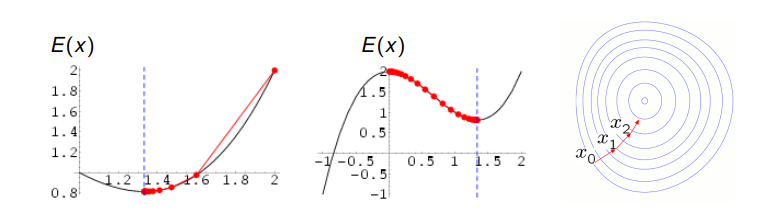
Gradient Descent or steepest descent is a first-order optimization method. It aims at computing a local minimum of a (generally) non-convex cost function by iteratively stepping in the direction in which the energy decreases most. This is given by the negative energy gradient.

To minimize a real-valued cost $E:\mathbb{R}^n\rightarrow \mathbb{R}$, the gradient flow for $E(x)$ is defined by the differential equation:

$$
\begin{cases}
x(0)=x_0 \\
\frac{dx}{dt} = \frac{dE}{dx}(x)
\end{cases}
$$
Discretization: $x_{k+1} = x_k -\epsilon\frac{dE}{dx}(x_k), \quad k=0,1,2,…$

Under certain conditions on $E(x)$, the gradient descent iteration:

$$
x_{k+1} = x_k - \epsilon \frac{dE}{dx}(x_k), \quad k=0,1,2…
$$

converges to a local minimum. For the case of concex $E$, this will also be the global minimum. The step size $\epsilon$ can be chosen differentlyin each iteration.

Gradient descent is a popular and broadly applicable method. It is typically not the fastest solution to compute minimizers because the asymptotic convergences rate is often inferior to that of more specialized algorithms. First-order methods with optimal convergence rates were pioneered by Yuri Nesterov.

In particular, highly anisotropic cost functions (with strongly different curvatures in different directioons) requires many iterations and trajectories tends to zig-zag. Locally optimal step sizes in each iteration can be computed by line search. For specific cost functions, alternative techniques such as the conjugate gradient method, Newton methods, or the BFGS method are preferable.

7.8 Linear Least Squares Estimation

Ordinary least squares or linear least squares is a method to for estimating a set of parameters $x \in \mathbb{R}^d$ in a linear regression model. Assume for each input vector $b_i\in \mathbb{R}^d, i\in {1, …,n}$, we observe a scalar response $a_i\in \mathbb{R}$. Assume there is a linear relationship of the form:

$$
a_i = b_i^\top x + \eta_i
$$

with an unknown vector $x\in \mathbb{R}^d$ and zero-mean Gaussian noise $\eta \sim \mathcal{N}(0, \mathbf{\Sigma})$ with a diagonal covariance matrix of the form $\mathbf{\Sigma }=\sigma^2\textbf{I}_n$. Maximum likelihood estimation of $x$ leads to the ordinary least squares problem:

$$
\min_{x}\sum_i (a_i -x^\top b_i)^2 = (a-\textbf{B}x)^\top(a-\textbf{B}x).
$$

Linear least squares estimation was introduced by Legendre (1805) and Gauss (1795/1809). When asking for which noise distribution the optimal estimator was the arithmetic mean, Gauss invented the normal distribution.

For general $\Sigma$, we get the generalized least squares problem:

$$
\min_{x} (a-\textbf{B}x)^\top \mathbf{\Sigma}^{-1}(a-\textbf{B}x).
$$

This is a quadratic cost function with positive definite $\mathbf{\Sigma^{-1}}$. It has the closed-form solution:

$$
\hat{x} = \underset{x}{argmin} (a-\textbf{B}x)^\top \mathbf{\Sigma}^{-1}(a-\textbf{B}x) \=(\textbf{B}^\top \mathbf{\Sigma}^{-1}\textbf{B})^{-1}\textbf{B}^\top\mathbf{\Sigma}^{-1}a.
$$

If there is no correlation among the observed variances, then the matrix $\mathbf{\Sigma}$ is diagonal. This case is referred to as weighted least squares:

$$
\min_x \sum_i w_i(a_i -x^\top b_i)^2, \quad with \ w_i=\sigma_i^{-2}.
$$

For the case of unknown matrix $\mathbf{\Sigma}$, there exist iterative estimation algorithm such as feasible generalized least squares or iteratively reweighted least squares.

7.9 Iteratively Reweighted Least Squares

The method of iteratively reweighted least squares aims at minimizing generally non-convex optimization problems if the form:

$$
\min_x \sum_i w_i(x)|a_i - f_i(x)|^2,
$$

with some known weighting function $\textcolor{green}{w_i(x)}$. A solution is obtained by iterating the following problem:
$$
x_{t+1} = \underset{x}{argmax} \sum_i w_i(x_t)|a_i - f_i(x)|^2.
$$
For the case that $f_i$ is linear, i.e. $f_i(x)=x^\top b_i$, each subproblem:

$$
x_{t+1} = \underset{x}{argmax} \sum_i w_i(x_t)|a_i - x^\top b_i|^2
$$

is simply a weighted least squares problem that can be solved in closed form. Nevertheless, this iterative approach will generally not converge to a global minimum of the original (non-convex) problem.

7.10 Nonlinear Least Squares Estimation

Nonlinear Least squares estimation aims at fitting observations $(a_i, b_i)$ with a nonlinear model of the form $a_i\approx f(b_i, x)$ for some function $f$ parameterized with an unknown vector $x\in \mathbb{R}^d$. Minimizing the sum of squares error:

$$
\min_x \sum_i r_i(x)^2, \quad with \ r_i(x) = a_i - f(b_i, x),
$$

is generally a non-convex optimization problem (因为函数f是非线性函数).

The optimality condition is given by:

$$
\sum_i r_i \frac{\partial r_i}{\partial x_j} = 0, \quad \forall j\in {1,…,d}.
$$

Typically one cannot directly solve these equation. Yet, there exist iterative algorithms for computing approximates solutions, including Netwon methods, the Gauss-Netwon algorithm and the Levenberg-Marquardt algorithm.

7.11 Newton Methods for Optimization

Netwon methods are second order methods: In constrast to first-order methods like gradient descent, they also make use of second derivatives. Geometrically, Netwon method iteratively approximately the cost function $E(x)$ quadratically and takes a step to the minimizer of this approximation.

Let $x_t$ be the estimated solution after $t$ iterations. Then the Talyor approximation of $E(x)$ in the vincinity of this estimate is:

$$
E(x) = E(x_t) + g^\top(x-x_t) + \frac{1}{2}(x-x_t)^\top \textbf{H}(x-x_t).
$$

The first and second derivative are denoted by the Jacobian $\textcolor{green}{g=\frac{dE}{dx}(x_t)}$ and the Hessian matrix $\textcolor{green}{\frac{d^2 E}{dx^2}(x_t)}$. For this second-order approximation, the optimality condition is:

$$
\frac{dE}{dx} = g + \textbf{H}(x-x_t) = 0
$$

Setting the next iterate to the minimizer $x$ leads to:

$$
x_{t+1} = x_t - \textbf{H}^{-1}g.
$$

In practice, one often choses a more conservative step size $\gamma \in (0, 1)$:

$$
x_{t+1} = x_t -\gamma \textbf{H}^{-1}g.
$$

When applicable, second-order methods are often faster than first-order methods, as least when measured in number of iterations. In particular, there exists a local neighborhood around each optimum where the Newton method converges quadratically for $\gamma = 1$ (if the Hessian is invertible and Lipschitz continuous).

For large optimization problems, computing and inverting the Hessian may be challenging. Moreover, since this problem is often not parallelizable, some second order methods do not profit from GPU acceleration. In such cases, one can aim to iteratively solve the extremality condition (*).

In case that $\textbf{H}$ is not positive definite, there exist quasi-Newton methods which aim at approximating $\textbf{H}$ or $\textbf{H}^{-1}$ with a positive definite matrix.

7.12 The Gauss-Newton Algorithm

The Gauss-Newton algorithm is a method to solve non-linear least-squares problems of the form:

$$
\min _x \sum_i r_i(x)^2.
$$

It can be derived as an approximation to the Newton method. The latter iterates:

$$
x_{t+1} = x_t - \textbf{H}^{-1}g.
$$

with the gradient $g$:

$$
g_j = 2\sum_i r_i\frac{\partial r_i}{\partial x_j},
$$

and the Hessian $\textbf{H}$:

$$
H_{jk} = 2\sum_i (\frac{\partial r_i}{\partial x_j}\frac{\partial r_i}{\partial x_k} + r_i\frac{\partial^2 r_i}{\partial x_j \partial x_k}).
$$

Dropping the second order term leads to the approximation:

$$
H_{jk} \approx 2 \sum_i J_{ij}J_{ik}, \quad with \ J_{ij} = \frac{\partial r_i}{\partial x_j}. (当我们假设误差函数near linear时，用近似的H才会有比较好的效果。)
$$

The approximation:

$$
\textbf{H} \approx 2J^\top J, \ with \ the \ Jacobin \textbf{J} = \frac{dr}{dx},
$$

together with $g = \textbf{J}^\top r$, leads to the Gauss-Netwon algorithm:

$$
x_{t+1} = x_t + \bigtriangleup, \quad with \ \bigtriangleup = -(\textbf{J}^\top \textbf{J})^-1\textbf{J}^\top r
$$

In contrast to the Newton algorithm, the Gauss-Newton algorithm does not require the computation of second derivatives. Moreover, the above approxamation of the Hessian is by construction positive definite.

This approximation of the Hessian is valid if:

$$
|r_i\frac{\partial ^2 r_i}{\partial x_j \partial x_k}| \ll |\frac{\partial r_i}{\partial x_j}\frac{\partial r_i}{\partial x_k}|,
$$

This is the case if the residuum $r_i$ is small or if it is close to linear (in which case the second derivatives are small).

7.13 The Levenberg-Marquardt Algorithm

The Newton algorirhm:

$$
x_{t+1} = x_t - \textbf{H}^{-1}g,
$$

can be modified (damped):

$$
x_{t+1} = x_t - (\textbf{H}+ \lambda \textbf{I}_n)^{-1}g,
$$

to create a hybrid between the Netwon method $\textcolor{green}{\lambda=0}$ and a gradient method with step size $\frac{1}{\lambda}$ (for $\textcolor{green}{\lambda \rightarrow \infty}$).

In the same manner, Levenberg (1944) suggested to damp the Gauss-Newton algorithm for nonlinear least squares:

$$
x_{t+1} = x_t + \bigtriangleup, \quad with \ \bigtriangleup=-(\textbf{J}^\top \textbf{J} + \lambda \textbf{I}_n)^{-1}\textbf{J}^\top r.
$$

Marquardt (1963) suggested a more adaptive component-wise damping of the form:

$$
\bigtriangleup = -(\textbf{J}^\top \textbf{J} + \lambda diag(\textbf{J}^\top \textbf{J}))^{-1}\textbf{J}^\top r,
$$

which avoids slow convergence in directions of small gradient.

7.14 Summary

Bundle adjustment was pioneered in the 1950s as a technique for structure and motion estimation in noisy real-world conditions. It aims at estimating the locations of $N$ 3D points $\textbf{X}_j$ and camera motions $(R_i, T_i)$, given noisy 2D projections ${\tilde{\textbf{x}}_i^j}$ in $m$ images.

The assumation of zero-mean Gaussian noise on the 2D observations leads to the weighted nonlinear least squares problem:

$$
E({R_i, T_i}_{i=1,…,m}, {\textbf{X}_j}_{j=1,…,N}) = \textcolor{green}{\sum_{i=1}^m}\sum_{j=1}^N \theta_{ij}|{\tilde{\textbf{x}}}_i^j - \pi(R_i,T_i, \textbf{X}_j)|^2,
$$

with $\textcolor{green}{\theta_{ij}=1}$ if point $j$ is visible in image $i$, $\theta_{ij}=0$ else.

Solutions of this non-convex problem can be computed by various iterative algorithms, most importantly a damped version of the Gauss-Newton algorithm called Levenberg-Marquardt algorithm. Bundle adjustment is typically initialized by an algorithm such as the 8-point or 5-point algorithm.