Chapter6 Reconstruction from Multiple Views

6.1 Multiple View Geometry

In this section, we deal with the problem of 3D reconstruction given multiple views of a static scene, either obtained simultaneously, or sequentially from a moving camera.
The key idea is that the three-view scenario allows to obtain more measurements to infer the same number of 3D coordinates. For example, given two views of a single 3D point, we have four measurements (x- and y-coordinate in each view), while the three-view case provides 6 measurements per point correspondence. As a consequence, the estimation of motion and structure will generally be more constrained when reverting to additional views.
The three-view case has traditionally been addressed by the so-called trifocal tensor [Hartley ’95, Vieville ’93] which generalizes the fundamental matrix. This tensor – as the fundamental matrix – does not depend on the scene structure but rather on the inter-frame camera motion. It captures a trilinear relationship between three views of the same 3D point or line [Liu, Huang ’86, Spetsakis, Aloimonos ’87].

6.2 Trifocal Tensor versus Multiview Matrices

Traditionally the trilinear relations were captured by generalizing the concept of the Fundamental Matrix to that of a Trifocal Tensor. It was developed among others by [Liu and Huang ’86], [Spetsakis, Aloimonos ’87]. The use of tensors was promoted by [Vieville ’93] and [Hartley ’95]. Bilinear, trilinear and quadrilinear constraints were formulated in [Triggs ’95]. This line of work is summarized in the books: Faugeras and Luong, “The Geometry of Multiple Views”, 2001 and Hartley and Zisserman, “Multiple View Geometry”, 2001, 2003.
In the following, however, we stick with a matrix notation for the multiview scenario. This approach makes use of matrices and rank constraints on these matrices to impose the constraints from multiple views. Such rank constraints were used by many authors, among others in [Triggs ’95] and in [Heyden, Åström ’97]. This line of work is summarized in the book Ma, Soatto, Kosecka, Sastry, “An Invitation to 3D Vision”, 2004.

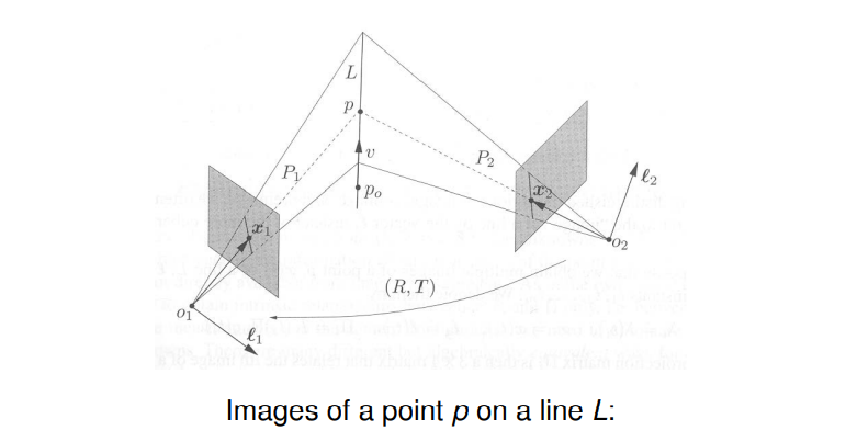
6.3 Preimage from Multiple Views

A preimage of multiple images of a point or a line is the (largest) set of 3D points that gives rise to the same set of multiple images of the point or the line.
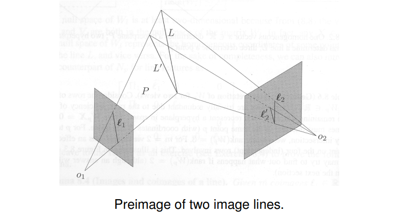
For example, given the two images $\ell_1$ and $\ell_2$ of a line $L$, the preimage of these two images is the intersection of the planes $P_1$ and $P_2$, i.e. exactly the 3D line $L = P_1\cap P_2$.

In general, the preimage of multiple images of points and lines can be defined by the intersection:

$$
preimage(\textbf{x}_1,…,\textbf{x}_m)=preimage(\textbf{x}_1)\cap …\cap preimage(\textbf{x}_m),\
preimage(\ell_1,…,\ell_m)=preimage(\ell_1)\cap …\cap preimage(\ell_m).\
$$

The above definition allows us to compute preimages for any set of image points or lines. The preimage of multiple image lines, for example, can be either an empty set, a point, a line or a plane, depending on whether or not they come from the same line in space.

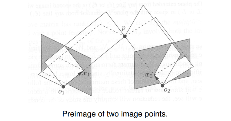
6.4 Preimage and Coimage of Points and Lines

Preimages $P_1$ and $P_2$ of the image lines should intersect in the line $L$.
Preimages of the two image points $\textbf{x}_1$ and $\textbf{x}_2$ should intersect in the point $p$.
Normals $\ell_1$ and $\ell_2$ define the coimages of the line $L$.

6.5 Preimage and Coimage of Points and Lines

For a moving camera at time $t$, let $\textbf{x}(t)$denote the image coordinates of a 3D point $\textbf{X}$ in homogeneous coordinates:

$$
\lambda(t)\textbf{x}(t) = K(t)\Pi_0 g(t)\textbf{X},
$$

where $\lambda (t)$ denotes the depth of the point, $K(t)$ denotes the intrinsic parameters, $\Pi_0$ the generic projection, and

$$
g(t) = \left(\begin{matrix}
R(t) &T(t)\\
0 & 1
\end{matrix} \right)\in SE(3),
$$

denotes the rigid body motion at time $t$.

Let us consider a 3D line $L$ in homogeneous coordinates:

$$
L = \{\textbf{X} |\textbf{X}=\textbf{X}_0 + \mu \textbf{V}, \mu \in \mathbb{R} \} \subset \mathbb{R}^4
$$

where $\textbf{X}_0=[X_0, Y_0, Z_0, 1]^T\in \mathbb{R}^4$ are the coordinates of the base point $p_0$ and $\textbf{V} =[V_1, V_2, V_3, 0]^T \in \mathbb{R}^4$ is a nonzero vector indicating the line direction.

The preimage of $L$ with respect to the image at time $t$ is a plane $P$ with normal $\ell(t)$, where $P=span(\hat{\ell})$. The vector $\ell(t)$ is orthogonal to all points $\textbf{x}(t)$ of the line:

$$
\ell (t)^T\textbf{x}(t) = \ell(t)^TK(t)\Pi_0 g(t)\textbf{X} =0.
$$

Assume we are given a set of $m$ images at times $t_1, …, t_m$ where:

$$
\lambda_i = \lambda(t_i), \textbf{x}_i = \textbf{x}(t_i), \quad \ell_i = \ell(t_i), \Pi_i = K(t_i)\Pi_0 g(t_i).
$$

With this notation, we can relate the i-th image of a point $p$ to its world coordinates $\textbf{X}$:

$$
\lambda_i \textbf{x}_i = \Pi_i \textbf{X},
$$

and the i-th coimage of a line $L$ to its world coordinates $(\textbf{X}_0, \textbf{V})$:

$$
\ell _i^T\Pi_i\textbf{X}_0 = \ell_i^T\Pi_i \textbf{V} = 0.
$$

6.6 From Preimages to Rank Constraints

The above equations contain the 3D parameters of points and lines as unknowns. As in the two-view case, we wish to eliminate these unknowns so as to obtain relationships between the 2D projections and the camera parameters.
In the two-view case an elimination of the 3D coordinates lead to the epipolar constraint for the essential matrix E or (in the uncalibrated case) the fundamental matrix F. The 3D coordinates (depth values $\lambda_i$ associated with each point) could nsubsequently obtained from another constraint.
There exist different ways to eliminate the 3D parameters leading to different kinds of constraints which have been studied in Computer Vision.
A systematic elimination of these constraints will lead to a complete set of conditions.

6.7 Point Features

Consider images of a 3D point $\textbf{X}$ seen in multiple views:

$$
\mathcal{I}\vec{\lambda} \equiv \left(\begin{matrix}
\textbf{x}_1 & 0 & \dots & 0\\
0 &\textbf{x}_2 & 0 & 0\\
\vdots &\vdots &\dots &\vdots \\
0 &0 &\dots &\textbf{x}_m
\end{matrix}\right)
\left(\begin{matrix}
\lambda_1\\
\lambda_2\\
\vdots \\
\lambda_m
\end{matrix}\right)=
\left(\begin{matrix}
\Pi_1\\
\Pi_2\\
\vdots \\
\Pi_m
\end{matrix}\right)\textbf{X} \equiv \Pi\textbf{X}.
$$

which is of the form:

$$
\mathcal{I}\vec{\lambda} = \Pi \textbf{X},
$$

where $m$ is the number of views, $\vec{\lambda}\in \mathbb{R}^m$ is the depth scale vector and $\Pi \in\mathbb{R}^{3m\times 4}$ the multiple-view projection matrix associated with the image matrix $\mathcal{I}\in \mathbb{R}^{3m\times m}$.

(Note:我们有$\mathcal{I}\vec{\lambda}=\Pi \textbf{X}$, 也就是$\Pi \textbf{X} - \mathcal{I}\vec{\lambda}=0$，即为$( \Pi, \mathcal{I})(\textbf{X}, \vec{-\lambda})^T = 0$,因此下文中要研究$N_p\equiv(\Pi, \mathcal{I})$的秩。)

Every column of $\mathcal{I}$ lies in a four-dimensional space spanned by columns of the matrix $\Pi$. In order to have a solution to the above equation, the columns of $\mathcal{I}$ and $\Pi$ must therefore be linearly dependent. In other words, the matrix:

$$
N_p \equiv (\Pi, \mathcal{I}) = \left(
\begin{matrix}
\Pi_1 &\textbf{x}_1 &0 &\dots &0 \\
\Pi_2 &0 &\textbf{x}_2 &0 &0\\
\vdots &\vdots &\vdots &\ddots &\vdots \\
\Pi_m &0 &0 &\dots &\textbf{x}_m
\end{matrix}\right) \in \mathbb{R}^{3m\times (m+4)}
$$

must have a nontrivial right null space. For $m \geq 2$ (i.e. $3m\geq m+4$), full rank would be $m+4$. Linear dependence of columns therefore implies the rank constraint:

$$
rank(N_p) \leq m+3.
$$

In fact, the vector $u = (\textbf{X}^T, -\vec{\lambda}^T)^T\in\mathbb{R}^{m+4}$ is the right null space, as $N_p u = 0.$

For a more compact formulation of the above rank constraint, we introduce the matrix:

$$
\mathcal{I}^\perp \equiv \left(
\begin{matrix}
\widehat{\textbf{x}_1} &0 &\dots &0\\
0 &\widehat{\textbf{x}_2} &\dots &0\\
\vdots &\vdots &\ddots &\vdots \\
0 &0 &\dots &\widehat{\textbf{x}_m}
\end{matrix}\right) \in \mathbb{R}^{3m\times 3m},
$$

which has the property of “annihilating” $\mathcal{I}$:

$$
\mathcal{I}^{\perp} \mathcal{I} = 0,
$$

we can premultiply the above equation to obtain:

$$
\mathcal{I}^{\perp} \Pi \textbf{X} = 0.
$$

(Note:我们有$\mathcal{I}\vec{\lambda}=\Pi \textbf{X}$, 两边同时左乘$\mathcal{I}^\perp就得到了上式$。)

Thus the vector $\textbf{X}$ is in the null space of the matrix:

$$
W_p \equiv \mathcal{I}^\perp \Pi = \left( \begin{matrix}
\widehat{\textbf{x}_1}\Pi_1\\
\widehat{\textbf{x}_2}\Pi_2\\
\vdots \\
\widehat{\textbf{x}_m}\Pi_m
\end{matrix}\right) \in \mathbb{R}^{3m\times 4}.
$$

To have a nontrivial solution(非平凡解), we must have:

$$
rank(W_p) \leq 3.
$$

If all images $\textbf{x}_i$ are from a single 3D point $\textbf{X}$, then the matrix $W_p$ should only have a one-dimensional null space. Given $m$ images $\textbf{x}_i\in \mathbb{R}^3$ of a point $p$ with respect to $m$ camera frames $\Pi_i$, we must have the rank condition:

$$
rank(W_p) = rank(N_p)-m \leq 3.
$$
(Note: 如果秩等于4，则所求问题无解，只有零解。如果秩为3，则所求问题有唯一非平凡解，如果秩小于3，则所求问题的解不唯一。)

6.8 Line Features

We can derive a similar rank constraint for lines. As we saw above, for the coimages $\ell_i, i=1,…,m$ of a line $L$ spanned by a base $\textbf{X}_0$ and a direction $\textbf{V}$ we have: ($\ell_i$ 是preimage的法向量)

$$
\ell_i^\top \Pi_i \textbf{X}_0 = \ell^\top_i\Pi_i\textbf{V} = 0.
$$

Therefor the matrix:

$$
W_l \equiv \left(\begin{matrix}
\ell^\top_1\Pi_1\\
\ell^\top_2\Pi_2\\
\vdots \\
\ell^\top_m\Pi_m
\end{matrix}\right) \in \mathbb{R}^{m\times 4}
$$

must satisfy the rank constraint:

$$
rank(W_l) \leq 2,
$$

since the null space of $W_l$ contains the two vectors $\textbf{X}_0$ and $\textbf{V}$.

6.9 Rank Consraints: Geometric Interpretation

In the case of a point $\textbf{X}$, wee had the equation:

$$
W_p\textbf{X} =0, \quad with \ W_p=\left(\begin{matrix}
\widehat{\textbf{x}_1}\Pi_1 \\
\widehat{\textbf{x}_2}\Pi_2 \\
\vdots \
\widehat{\textbf{x}_m}\Pi_m
\end{matrix}\right) \in \mathbb{R}^{3m \times 4}.
$$

Since all matrices $\hat{\textbf{x}}_i$ have rank 2, the number of independent rows in $W_p$ is at most $2m$. These rows define a set of $2m$ planes.

(Note: $\hat{\textbf{x}}_i$ 是$\textbf{x}_i$的反对称矩阵，且因为其cross的性质，使得$\hat{\textbf{x}_i}\textbf{x}_i=0$,因此可以看作是秩为2的反对称矩阵中含了两个法向量，与这这两个法向量对应的垂直平面中有点$\textbf{x}_i$，因此一个反对称矩阵中就定义了2个平面，那么m个views下总共就包含了$2m$个平面。)

Since $W_p\textbf{X}=0$, the point $\textbf{X}$ is in the intersection of all these planes. In order for the $2m$ planes to have a unique intersection, we need to have $rank(W_p)=3$.

The rows of the matrix $W_p$ correspond to the normal vectors of four planes. The (nontrivial) rank constraint states that these four planes have to intersect in a single point.

In the case of a line $L$ in two views, we have the equation:

$$
rank(W_l)\leq 2, \quad \ W_l = \left(
\begin{matrix}
\ell^\top_1\Pi_1 \\
\ell^\top_2\Pi_2
\end{matrix}\right) \in \mathbb{R}^{2\times 4}.
$$

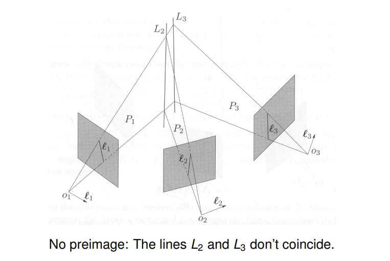
Clearly, we already have $rank(W_l)\leq 2$, so there is no intrinsic constraint on two images of a line: The preimage o two image lines always contains a line. We shall see that this is no longer true for three or more images of a line, then the above constraint really becomes meaningful.

For the case of a line observed from two images, the rank constraint is always fulfilled. Geometrically this ststes that the two preimages of each line always intersect in some 3D line.

6.9 The Multiple-view Matrix of a Point

In the following, the rank constraints will be rewritten in a more compact and transparent manner. Let us assume we have $m$ images, the first of which is in world coordinates. Then we have projection matrices of the form:

$$
\Pi_1 = [I, 0], \ \Pi_2=[R_2, T_2], \ …, \ \Pi_m=[R_m,T_m] \in \mathbb{R}^{3\times 4},
$$

which model the projection of a point $\textbf{X}$ into the individual images.

In general for uncalibrated cameras (i.e. $K_i\neq I$), $R_i$ will not be an orthogonal rotation matrix but rather an arbitrary invertible matrix.

Again, we define the matrix $W_p$ as follows:

$$
W_p = \mathcal{I}^{\bot}\Pi = \left(
\begin{matrix}
\widehat{\textbf{x}_1}\Pi_1 \\
\widehat{\textbf{x}_2}\Pi_2 \\
\vdots \
\widehat{\textbf{x}_m}\Pi_m
\end{matrix}\right)\in \mathbb{R}^{3m\times 4}.
$$

The rank of the matrix $W_p$ is not affected if we multiply by a full-rank matrix $D_p\in \mathbb{R}^{4\times 5}$ as follows:

$$
W_pD_p = \left(
\begin{matrix}
\widehat{\textbf{x}_1}\Pi_1 \\
\widehat{\textbf{x}_2}\Pi_2 \\
\vdots \\
\widehat{\textbf{x}_m}\Pi_m
\end{matrix}\right)
\left(
\begin{matrix}
\widehat{\textbf{x}_1} &\textbf{x}_1 &0\\
0 &0 &1
\end{matrix}\right)=
\left(
\begin{matrix}
\widehat{\textbf{x}_1}\widehat{\textbf{x}_1} &0 &0 \\
\widehat{\textbf{x}_2}R_2\widehat{\textbf{x}_1} &\widehat{\textbf{x}_2}R_2\textbf{x}_1 &\widehat{\textbf{x}_2}T_2 \\
\widehat{\textbf{x}_3}R_3\widehat{\textbf{x}_1} &\widehat{\textbf{x}_3}R_3\textbf{x}_1 &\widehat{\textbf{x}_3}T_3 \\
\vdots &\vdots &\vdots \\
\widehat{\textbf{x}_m}R_m\widehat{\textbf{x}_1} &\widehat{\textbf{x}_m}R_m\textbf{x}_1 &\widehat{\textbf{x}_m}T_m
\end{matrix}\right)
$$

This means that $rank(W_p)\leq 3$ if and only if the submatrix:

$$
M_p = \left(
\begin{matrix}
\widehat{\textbf{x}_2}R_2\textbf{x}_1 &\widehat{\textbf{x}_2}T_2 \\
\widehat{\textbf{x}_3}R_3\textbf{x}_1 &\widehat{\textbf{x}_3}T_3 \\
\vdots &\vdots \
\widehat{\textbf{x}_m}R_m\textbf{x}_1 &\widehat{\textbf{x}_m}T_m
\end{matrix}\right) \in \mathbb{R}^{3(m-1)\times 2 }
$$

has $rank(M_p)\leq 1$.

The matrix

is called the multiple-view matrix associated with a point $p$. It involves both the image $\textbf{x}_1$ in the first view and the coimages ${\widehat{\textbf{x}}}_i$ in the remaining views.

In summary:
For multiple images of a point $p$ the matrices $N_p, W_p, M_p$ satisfy:

$$
rank(M_p) = rank(W_p)-2 = rank(N_p)-(m+2) \leq 1.
$$

6.10 Multiview Matrix: Geometric Interpretation

Let us look into the geometric information contained in the multiple-view matrix:

$$
M_p = \left(
\begin{matrix}
\widehat{\textbf{x}_2}R_2\textbf{x}_1 &\widehat{\textbf{x}_2}T_2 \\
\widehat{\textbf{x}_3}R_3\textbf{x}_1 &\widehat{\textbf{x}_3}T_3 \\
\vdots &\vdots \\
\widehat{\textbf{x}_m}R_m\textbf{x}_1 &\widehat{\textbf{x}_m}T_m
\end{matrix}\right) \in \mathbb{R}^{3(m-1)\times 2 }.
$$

The constraint $rank(M_p)\leq 1$ implies that the two columns are linearly dependent. In fact that we have:
$\lambda_1\widehat{\textbf{x}_i}R_i\textbf{x}_i + \widehat{\textbf{x}_i}T_i = 0, i=2, …,m$ which yields:

$$
M_p\left(\begin{matrix}
\lambda_1 \\
1
\end{matrix}\right) = 0.
$$

Therefore the coefficient capturing the linear dependence is simply the distance $\lambda_1$ of the point $p$ from the first camera center. In other words, the multiple-view matrix captures exactly the information about a point $p$ that is missing from a single image, but encoded in multiple images.

6.11 Relation to Epipolar Constraints

For the multiple-view matrix:

$$
M_p = \left(
\begin{matrix}
\widehat{\textbf{x}_2}R_2\textbf{x}_1 &\widehat{\textbf{x}_2}T_2 \\
\widehat{\textbf{x}_3}R_3\textbf{x}_1 &\widehat{\textbf{x}_3}T_3 \\
\vdots &\vdots \\
\widehat{\textbf{x}_m}R_m\textbf{x}_1 &\widehat{\textbf{x}_m}T_m
\end{matrix}\right) \in \mathbb{R}^{3(m-1)\times 2 }.
$$

to have $rank(M_p)=1$, it is necessary that the pair of vectors $\widehat{\textbf{x}_i}T_i$ and $\widehat{\textbf{x}}_iR_i\textbf{x}_1$ to be linearly dependent for all $i=2,…,m$. This gives the epipolar constraints:

$$
\textbf{x}_i^{\top}\widehat{T_i}R_i \textbf{x}_1 = 0
$$

between the first and $i$-th image.
Yet, we shall see that the multiview constraint provides more information than the pairwise epipolar constraints.

We claimed that the linear dependence of $\widehat{\textbf{x}_i}T_i$ and $\widehat{\textbf{x}_i}R_i\textbf{x}_1$ gives rise to the epipolar constraint $\textbf{x}_i^\top \widehat{T_i}R_i\textbf{x}_1 =0$. In the following, we shall give a proof of this statement which provides an intuitive geometric understanding of this relationship.

Assume the two vectors $\widehat{\textbf{x}_i}T_i$ and $\widehat{\textbf{x}_i}R_i\widehat{\textbf{x}_1}$ are dependent, i.e. there is a scalar $\gamma$, such that

$$
\widehat{\textbf{x}_i}T_i = \gamma \widehat{\textbf{x}_i}R_i\textbf{x}_1.
$$

Since $\widehat{\textbf{x}_i}T_i \equiv \textbf{x}_i\times T_i$ is proportational to the normal on the plane spanned by $\textbf{x}_i$ and $T_i$, and $\widehat{\textbf{x}_i}R_i\textbf{x}_1$ is proportational to the normal spanned by $\textbf{x}_i$ and $R\textbf{x}_1$, the linear dependence is equivalent to saying that the three vectors $\textbf{x}_i, T_i$ and $R_i\textbf{x}_1$ are coplanar. (Note: $\widehat{\textbf{x}_i}$ 和$T_i$叉乘后的向量与$\widehat{\textbf{x}_i}$ 和$R_i\textbf{x}_1$叉乘后的向量同向且相差一个尺度系数，说明向量$\widehat{\textbf{x}_i}, T_i, R_i\textbf{x}_1$是共平面的，也就有了下面所说的$\widehat{\textbf{x}_i}$与平面的法向量正交。)

This again is equivalent to saying that the vector $\textbf{x}_i$ is orthogonal to the normal on the plane spanned by the vectors $T_i$ and $R_i\textbf{x}_1$, i.e.

$$
\widehat{\textbf{x}_i}^\top(T_i \times R_i\textbf{x}_1) = \widehat{\textbf{x}_i}^\top \widehat{T}_iR_i\textbf{x}_1 = 0.
$$

6.12 Analysis of the Multiple-view Constraint

For any nonzero vectors $a_i, b_i\in \mathbb{R}^4, i=1,2,…,n$, the matrix

$$
\left(\begin{matrix}
a_1 &b_1\\
a_2 &b_2\\
\vdots &\vdots \\
a_n &b_n
\end{matrix}\right) \in \mathbb{R}^{3n\times 2}
$$

is rank-deficient if and only if $a_ib_j^T-b_ia_j^T = 0$ for all $i,j=1,…,n$. We will not prove this statement. Applied to the rank constraint on $M_p$ we get:

$$
\widehat{\textbf{x}_i}R_i\textbf{x}_1(\widehat{\textbf{x}_j}T_j)^\top - \widehat{\textbf{x}_i}T_i(\widehat{\textbf{x}_j}R_j\textbf{x}_1)^\top = 0,
$$

which gives the trilinear constraint:

$$
\widehat{\textbf{x}_i}(T_i\textbf{x}_1^\top R_j^\top - R_i\textbf{x}_1T_j^\top)\widehat{\textbf{x}_j} = 0.
$$

This is a matrix equation giving $3\times 3=9$ scalar trilinear equations, only four of which are linearly independent.

From the equations:

$$
\widehat{\textbf{x}_i}R_i\textbf{x}_1(\textbf{x}_jT_j)^\top - \widehat{\textbf{x}_i}T_i(\widehat{\textbf{x}_j}R_j\textbf{x}_1)^\top = 0, \quad \forall i,j.
$$

we see that as long as the entries in $\widehat{\textbf{x}_j}T_j$ and $\widehat{\textbf{x}_j}R_j\textbf{x}_j$ are non-zero, it follows from the above, that the two vectors $\widehat{\textbf{x}_i}R_i\textbf{x}_1$ and $\widehat{\textbf{x}_i}T_i$ are linearly dependent. If on the other hand $\widehat{\textbf{x}_j}T_j = \widehat{\textbf{x}_j}R_j\textbf{x}_1=0$ for some view $j$, then we have the rare degenerate case that the point $p$ lies ont the line through the optical centers $o_1$ and $o_j$.

In other words: Except for degeneracies, the bilinear (epipolar) constrints relating two views are already contained in the trilinear constraints obtained for the multi-view scenario.

Note that the equivalence between the bilinear and trilinear constraints on one hand and the condition that $rank(M_p)\leq 1$ on the other only holds if the vectors in $M_p$ are nonzero. In certain degenerate cases this is not fulfilled.

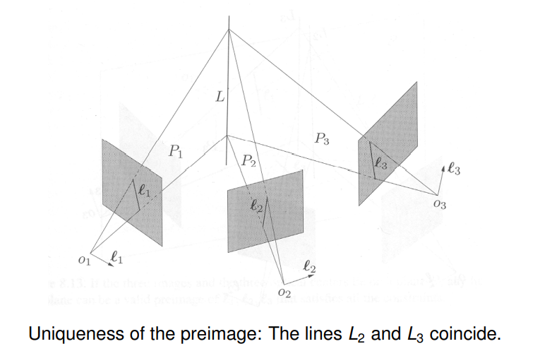
6.13 Uniqueness of the Preimage (Teacher skip this part…)

We will now clarify hoe the bilinear and trilinear constraints help to assure the uniqueness of the preimage of a point observed in three images.

Given three vectors $\textbf{x}_1, \textbf{x}_2, \textbf{x}_3\in \mathbb{R}^3$ and three camera frames with distinct optical centers, if the three images satisfy the pairwise epipolar constraints:

$$
\textbf{x}_i^\top \widehat{T_{ij}}R_{ij}\textbf{x}_j = 0, \quad i,j=1,2,3.
$$

then a unique preimage is determined except if the three lines associated to image points $\textbf{x}_1, \textbf{x}_2, \textbf{x}_3$ are coplanar.

Here $T_{ij}$ and $R_{ij}$ refer to the transition between frame $i$ and $j$.
Similarly, if these vectors satisfy all trilinear constraints:

$$
\widehat{\textbf{x}_i}(T_{ji}\textbf{x}_i^\top R_{ki}^\top - R_{ji}\textbf{x}_iT_{ki}^\top)\widehat{\textbf{x}_k} = 0, \quad i,j,k=1,2,3.
$$

then a unique preimage is determine unless the three lines associated to image points $\textbf{x}_1, \textbf{x}_2, \textbf{x}_3$ are colinear.

We will not prove these statement.(Note: F**k!)

6.14 Degeneracies for the Bilinear Constraints

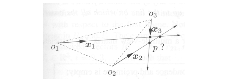
In the above example, the point $p$ lies in the plane spanned by the three optical centers which is also called the trifocal plane.

In this case, all points of lines do intersect, yet it does not imply a unique 3D point $p$ (a unique preimage). In practice this degenerate case arises rather seldom.

In the above example, the optical centers lie on a straight line (rectilinear motion). Again, all pairs of lilnes may intersect without there being a unique preimage $p$.

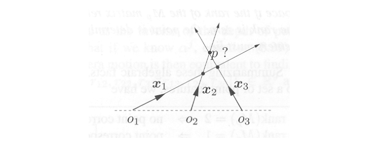
This case is frequent in applications when the camera moves in a straight line (e.g. a car on a highway). Then the epipolar constraints will not allow a unique reconstruction.

Fortunately, the trilinear constraint assures a unique preimage (unless $p$ is also on the same line with the optical centers).

6.15 Uniqueness of the Preimage

Using the multiple-view matrix we obtain a more general and simpler characterization regarding the uniqueness of the preimage.

Given $m$ vectors representing the $m$ images of a point in $m$ views, they correspond to the same point in the 3D space if the rank of the $M_p$ matrix relative to any of the camera frames is one. If the rank is zero, the point is determined up to the line on which all the camera centers must lie.

In summary we get:

$rank(M_p)=2 \Rightarrow$	no point correspondence & empty preimage
$rank(M_p)=1 \Rightarrow$	point correspondence & unique preimage
$rank(M_p)=0 \Rightarrow$	point correspondence & preimage not unique

With these constraints we could decide which features to match for establishing point correspodence over multiple frames.

6.16 Multiple-view Factorization of Point Features

The rank condition on the multiple-view matrix captures all the constraints among multiple images of a point. In principle, one could perform reconstruction by maximizing some global objective function subject to the rank condition. This would lead to a nonlinear optimization problem analogous to the bundle adjustment in the two-view case.
Alternatively, one can aim for a similar separation of structure and motion as done for the two-view case in the eight-point algorithm. Such an algorithm shall be detailed in the following.

One should point out that this approach does not necessarily lead to a practical algorithm as the spectral approaches do not imply optimality in the context of noise and uncertainty.

Suppose we have $m$ images $\textbf{x}_1^j, …, \textbf{x}_m^j$ of $n$ points $p^j$ and we want to estimate the unknown projection matrix $\Pi$.

The condition $rank(M_p)\leq 1$ states that the two columns of $M_p$ are linear dependent. For the $j$-th point $p^j$ this implies:

$$
\left(\begin{matrix}
\widehat{\textbf{x}_2^j}R_2\textbf{x}_1^j \\
\widehat{\textbf{x}_3^j}R_3\textbf{x}_1^j \\
\vdots \\
\widehat{\textbf{x}_m^j}R_m\textbf{x}_1^j \\
\end{matrix}\right) + \alpha^j \left(\begin{matrix}
\widehat{\textbf{x}_2^j}T_2 \\
\widehat{\textbf{x}_3^j}T_3 \\
\vdots \
\widehat{\textbf{x}_m^j}T_m \
\end{matrix}\right) = 0\in \mathbb{R}^{3(m-1)\times 1},
$$

for some parameters $\alpha ^j\in \mathbb{R}, j=1,…,n$. Each row in the above equation can be optained from $\lambda_i^j\textbf{x}_i^j = \lambda_1^j R_i\textbf{x}_1^j + T_i$, multiplying by $\widehat{\textbf{x}_i^j}$:

$$
\widehat{\textbf{x}_i^j}R_i\textbf{x}_1^j + \widehat{\textbf{x}_i^j}T_i/\lambda_1^j = 0.
$$

Therefore, $\lambda^j = 1/\lambda_1^j$ is nothing but the inverse of the depth of point $p^j$ with respect to the first frame.

6.17 Motion Estimation from Known Structure

Assume we have the depth of the points and thus their inverse $\alpha^j$ (i.e. known structure). Then the above equation is linear in the camera motion parameters $R_i$ and $T_i$. Using the stack notation $R_i^s=[r_{11}, r_{21}, r_{310}, r_{12}, r_{22}, r_{32}, r_{13}, r_{23}, r_{33}]^T \in \mathbb{R}^9$ and $T_i\in \mathbb{R}^3$, we have the linear equation system:

$$
P_i\left(\begin{matrix}
R_i^s\
T_i
\end{matrix}\right) = \left(\begin{matrix}
\textbf{x}_1^{1T}\otimes \widehat{\textbf{x}_i^1} &\alpha^1\widehat{\textbf{x}_i^1} \\
\textbf{x}_1^{2T}\otimes \widehat{\textbf{x}_i^2} &\alpha^2\widehat{\textbf{x}_i^2} \\
\vdots &\vdots \\
\textbf{x}_1^{nT}\otimes \widehat{\textbf{x}_i^n} &\alpha^n\widehat{\textbf{x}_i^n}
\end{matrix}\right)
\left(\begin{matrix}
R_i^s\\
T_i
\end{matrix}\right) = 0 \in \mathbb{R}^{3n}.
$$

One can show that the matrix $P_i\in \mathbb{R}^{3n\times 12}$ is of rank 11 if more than $n=6$ points in general position are given.
(Note:我们可以看到当有5对点时，$3n$就已经大于12了，但是反对称矩阵里面的秩为2，只有两行是线性无关的，因此$3n$行里面其实线性无关的只有$2n$行，因此当有超过6对点时，我们才能确保说$P_i$的秩为11时有唯一的解。)
In that case the null space of $P_i$ is onedimensional and the projection matrix $\Pi_i = (R_i, T_i)$ is given up to a scale factor. In practice one would use more than 6 points, obtain a full-rank matrix and compute the solution by a singular value decomposition (SVD).
(Note:可以明显看出，这个其实和典型的8点法还是有区别的，典型的8点法完全将motion和structure解耦开了，即估计相机motion的时候是不用知道任何结构的信息的，不管是3D的点也好，还是点的深度信息也好，都是不用知道的，但这里的8点法估计motion时，需要一个参数$\alpha^j $)，这个参数得事先知道。才能去估计相机的motion(R, T)，进而才能估计3D点的坐标，因此没有完全将motion和structure解耦开来。)

6.18 Structure Estimation from Known Motion

In turn, if the camera motion $\Pi_i = (R_i, T_i), i=1,2,…,m$ is known, we can estimate the structure (depth parameters $\alpha^j, j=1,…,m$). The least squares solution for the above equation is given by:

$$
\alpha_j = -\frac{\sum_{i=2}^m(\widehat{\textbf{x}_i^j}T_i)^\top \widehat{\textbf{x}_i^j}R_i\textbf{x}1^j}{\sum{i=2}^m ||\widehat{\textbf{x}_i^j}T_i||^2}, \quad j=1,2,…,n.
$$

In this way one can iteratively estimate structure and motion, estimating one while keeping the fixed.

For initialization one could apply the eight-point algorithm to the first two image to obtain an eatimate of the structure parameters $\alpha^j$.
(Note: 初始化的方案：先用两帧图像使用8点法去求解motion，进而估计structure，得到深度，然后在这个基础上使用multi-view的8点法进行估计motion，然后借由motion去优化$\alpha$,反复迭代motion与structure的求解。)

While the equation for $\Pi_i$ makes use of the two frames 1 and $i$ only, the structure parameter estimation takes into account all frames. This can be done either in batch mode or recursively.

As for the two-view case, such spectral approaches do not guarantee optimiality in the presence of noise and uncertainty.

6.19 Multiple-view Matrix for Lines

The matrix:

$$
W_l = \left(\begin{matrix}
\ell^\top_1\Pi_1 \\
\ell^\top_2\Pi_2 \\
\vdots \\
\ell^\top_m\Pi_m
\end{matrix}\right) \in \mathbb{R}^{m\times 4}
$$

associated with $m$ images of a line in space satisfies the rank constraint $rank(W_l)\leq 2$, because $W_l\textbf{X}_0 = W_l\textbf{V}=0$ for the base point $\textbf{X}_0$ and the direction $\textbf{V}$ of the line. To find a more compact representation, let us assume that the first camera is in world coordinates, i.e. $\Pi_1=(I,0)$. The rank is not affected by multiplying with a full-rank matrix $D_l\in \mathbb{R}^{4\times 5}$:

$$
W_lD_l = \left(\begin{matrix}
\ell_1^\top &0 \\
\ell^\top_2 R_2 &\ell^\top_2T_2\\
\vdots &\vdots \\
\ell^\top_mR_m &\ell^\top_mT_m
\end{matrix}\right)
\left(\begin{matrix}
\ell_1 &\widehat{\ell_1} &0 \\
0 &0 &1
\end{matrix}\right) =
\left(\begin{matrix}
\ell_1^\top\ell_1 &0 &0\\
\ell^\top_2R_2\ell_1 &\ell^\top_2R_2\widehat{\ell_1} &\ell^\top_2T_2 \\
\vdots &\vdots &\vdots\\
\ell^\top_mR_m\ell_1 &\ell^\top_mR_m\widehat{\ell_1} &\ell^\top_mT_m \\
\end{matrix}\right)
$$

Since multiplication with a full rank matrix does not affect the rank, we have:

$$
rank(W_lD_l) = rank(W_l) \leq 2.
$$

Since the first column of $W_lD_l$ is linearly independent from the remaining ones, the submatrix:

$$
\left(\begin{matrix}
\ell^\top_2R_2\widehat{\ell_1} &\ell^\top_2T_2 \\
\vdots &\vdots\\
\ell^\top_mR_m\widehat{\ell_1} &\ell^\top_mT_m \\
\end{matrix}\right) \in \mathbb{R}^{(m-1)\times 5},
$$

has the rank constraint:

$$
rank(M_l) \leq 1.
$$

(Note: 这个约束其实蛮strong的，一般我们使用multi-view进行重建时，$m$的取值会比较大，比如说是6，那么这种情况下得到的$5\times 5$的矩阵要保持秩小于1其实还挺难的)

For the case of a line projected into $m$ images, we have a much stronger rank-condtraint than in the case of a projected point:
For a sufficiently large number of views $m$, the matrix $M_l$ could in principle have a rank of five. The above constraint states that a meaningful preimage of $m$ observed lines can only exist if $rank(M_l)\leq 1$.

6.20 Trilinear Constraints for a Line

Again, we can take a closer look at the meaning of the above rank constraint. Regarding the first three columns of $M_l$ it implies that respective row vectors must be pairwise linearly dependent, i.e. for all $i,j\neq 1$:

$$
\ell^\top_1 R_i\widehat{\ell_1} \sim \ell_j^\top R_j\widehat{\ell_1},
$$

which is equivalent to the trilinear equation:

$$
\ell_iR_i\widehat{\ell_1}R^\top_j\ell_j = 0.
$$

Proof: The above proportionality states that the three vectors $R_i^\top\ell_i$, $R^\top_j\ell_j$ and $\ell_1$ are coplanar. The lower equation is the equivalent ststement that the vector $R_i^\top \ell_i$ is orthogonal to the normal on the plane spanned by $R_j^\top\ell_j$ and $\ell_1$.

Interestingly, the above constraint only involves the camera rotations, not the camera translations.

Taking into account the fourth column of the multiple-view matrix $M_l$, the rank constraint implies the linear dependency between the $i$-th and the $j$-th row. This is equivalent to the trilinear constraint:

$$
\ell_j^\top T_j\ell^\top _iR_i\widehat{\ell_1}-\ell_i^\top T_i\ell^\top _jR_j\widehat{\ell_1} = 0.
$$

The proof follows from the general analysis of the Multiple-view Constraint in ##6.12##.

The above constraint relates the first, the $i$-th and the $j$-th images. From previous discussion, we saw that all nontrivial constraints in the case of lines involve at least three images. The two trilinear constraints above are equivalent to the rank constraint if the scalar $\ell_i^\top T_i\neq 0$, i.e. in non-degenerate cases.

In general, $rank(M_l)\leq 1$ if and only if all its $2\times 2$-minors have zero determinant. Since these minors only include three images at a time, one can conclude that any multi-view constraint on lines can be reduced to constraints which only involve three lines at a time.

6.21 Uniqueness of the Preimage

The key idea to the rank constraint on the multiple-view matrix $M_l$ was to assure that $m$ observations of a line correspond to a consistent preimage $L$. The uniqueness of the preimage in the case of the trilinear constraints can be characterized as follows:

Lemma: Given three camera frames with distinct optical centers and any three vectors $\ell_1, \ell_2, \ell_3\in \mathbb{R}^3$ that represent three image lines. If the three image lines satisfy the trilinear consrraints:
$$\ell_j^\top T_{ji}R_{ki}\widehat{\ell_i} - \ell_k^\top T_{ki}\ell_j^\top R_{ji}\widehat{\ell_i}=0, \quad i,j,k\in {1,2,3}.$$
then their preimage $L$ is uniquely determined except for the case in which the preimage of every $\ell_i$ is the same plane in space. This is the only degenerate case, and in this case, the matrix $M_l$ becomes zero.

Note that the above constraint combines the two trilinear constraints introduced on the previous section.

A similar statement can be made regarding the uniqueness of the preimage of $m$ lines in relation to the rank of the multiview matrix $M_l$.

Theorem:
Given $m$ vectors $\ell_i \in \mathbb{R}^3$ representing images of lines with respect to $m$ camera frames. They correspond to the same line in space if the rank of the matrix $M_l$ relative to any of the camera frames is 1. If its rank is 0 (i.e. the matrixx $M_l$ itself is zero), then the line is determined up to a plane on which all the camera centers must lie.

Overall we have the following cases:

$rank(M_l)=2 \Rightarrow$	no line correspondence
$rank(M_l)=1 \Rightarrow$	line correspondence & unique preimage
$rank(M_l)=0 \Rightarrow$	line correspondence & preimage not unique (在第一张图片形成的preimage平面内translation camera而没有其他motion)

6.22 Summary

One can generalize the two-view scenario to that of simultaneously considering $m\geq 2$ images of a scene. The intrinsic constraints among multiple images of a point or a line can be expressed in terms of rank conditions on the matrix $N$, $W$ or $M$.

The relationship among these rank conditions is as follows:

	(Pre) image	coimage	Jointly
Point	$rank(N_p)\leq m+3$	$rank(W_p)\leq 3$	$rank(M_p)\leq 1$
Line	$rank(N_l)\leq 2m+2$	$rank(W_l)\leq 2$	$rank(M_l)\leq 1$

These rank conditions capture the relationship among corresponding geometric primitives in multiple images. They impose the existence of unique preimages (up to degenerate cases). Moreover, they give rise to natural factorization-based algorithm for multiview recovery of 3D structure and motion (i.e. generalizations of the 8-point algorithm).