Chapter 4 Estimating Point Correspondence

4.1 From Photometry to Geometry

In the last sections, we discussed how points and lines are transformed from 3D world coordinates to 2D image and pixel coordinates.

In practice, we do not actually observe points or lines, but rather brightness or color values at the individual pixels. In order to transfer from this photometric representation to a geometric representation of the scene, one can identify points with characteristic image features and try to associate these points with corresponding points in the other frames.

The matching of corresponding points will allow us to infer 3D structure. Nevertheless, one should keep in mind that this approach is suboptimal:By selecting a small number of feature points from each image, we throw away a large amount of potentially useful information contained in each image. Yet, retaining all image information is computationally challenging. The selection and matching of a small number of feature points, on the other hand, was shown to permit tracking of 3D objects from a moving camera in real time.

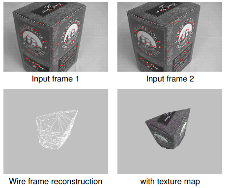
4.2 Example of tracking

4.3 Identifying Corresponding Points

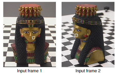
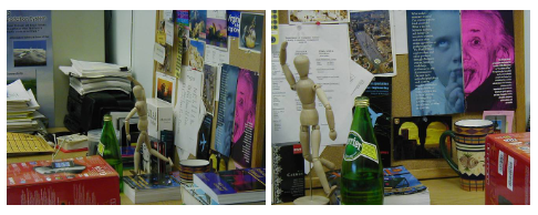
To identify corresponding points in two or more images is one of the biggest challenges in computer vision. Which of the points identified in the left image corresponds to which point in the right one?

4.4 Non-rigid Deformation

In what follows we will assume that objects move rigidly.
However, in general, objects may also deform non-rigid. Moreover, there may be partial occlusions: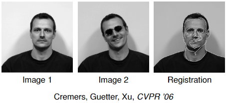

4.5 Small Deformation versus Wide Baseline

In point matching one distinguishes two cases:

Small deformation: The deformation from one frame to the other is assumed to be (infinitesimally) small. In this case the displacement from one frame to the other can be estimated by classical optical flow estimation, for example using the methods of Lucas/Kanade or Horn/Schunck. In particular, these methods allow to model dense deformation fields (giving a displacement for every pixel in the image). But one can also track the displacement of a few feature points which is typically faster.
Wide baseline stereo: In this case the displacement is assumed to be large. A dense matching of all points to all is in general computationally infeasible. Therefore, one typically selects a small number of feature points in each of the images and develops efficient methods to find an appropriate pairing of points.

4.6 Small Deformation

The transformation of all points of a rigidly moving obnect is given by: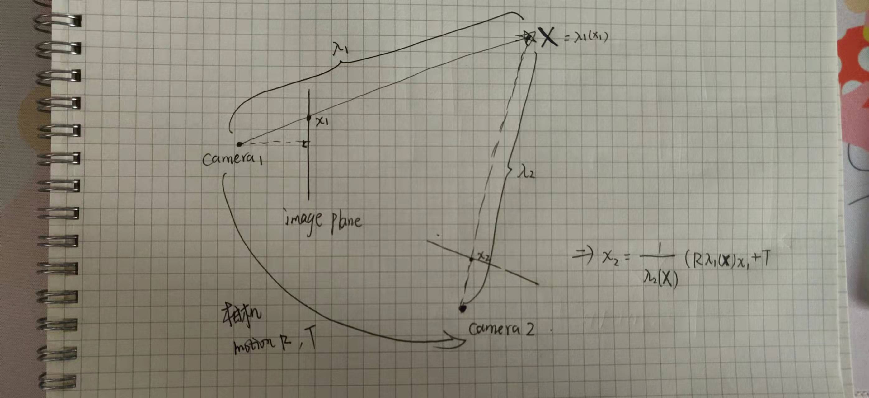

$$
x_2 = h(x_1) = \frac{1}{\lambda _2(\textbf{X})}(R\lambda_1(\textbf{X})x_1 + T).
$$

Locally this motion can be approximated in several ways.

Translational model:
$$
h(x) = x + b.
$$
Affine model:

$$
h(x) = Ax + b.
$$
The 2D affine model can also be written as:
$$h(x) = x + u(x)\quad (u就是像素从当前帧到下一帧中的运动) $$
with
$$
u(x) = S(x)p = \left(\begin{matrix}
x &y&1&0&0&0\\
0&0&0&x&y&1
\end{matrix}\right)(p_1, p_2, p_3,p_4,p_5,p_6)^T =
\left(\begin{matrix}
p_1x+p_2y+p_3\\
p_4x+p_5y+p_6
\end{matrix}\right).
$$

4.7 Optic Flow Estimation

The optic flow refers to the apparent 2D motion field observable between consecutive images of a video. It is different from the motion of objects in the scene, in the extreme case of motion along the camera axis, for example, there is no optic flow, while on the other hand camera rotation generates an optic flow field even for entirely static scenes.

In 1981, two seminal works on optic flow estimation were published, namely the works of Lucas & Kanade, and of Horn & Schunck. Both methods have become very influential with thousands of citations. They are complementary in the sense that the Lucas-Kanade method generates sparse flow vectors under the assumption of constant motion in a local neighborhood, whereas the Horn-Schunck method generates a dense flow field under the assumption of spatially smooth flow fields. Despite more than 30 years of research, the estimation of optic flow fields is still a highly active research direction.

4.8 The Lucas-Kanade Method

Brightness Constancy Assumption: Let $x(t)$ denote a moving point at time $t$, and $I(x,t)$ a video sequence, then:
$$
I(x(t), t) = const. \quad \forall t,
$$
i.e. the brightness of point $x(t)$ is constant. Then the total time derivative must be zero:
$$
\frac{d}{dt}I(x(t), t) = \nabla I^T(\frac{dx}{dt}) + \frac{\partial I}{\partial t} = 0.
$$
This constraint is often called the (different) optical flow constraint. The desired local flow vector (velocity) is given by $v = \frac{dx}{dt}$.
Constant motion in a neighborhood: Since the above equation cannot be solved for $v$, one assumes that $v$ is constant over a neighborhood $W(x)$ of the point $x$:
$$
\nabla I(x’, t)^T v + \frac{\partial I}{\partial t}(x’, t) = 0 \quad \forall x’ \in W(x).
$$

The brightness is typically not exactly constantly and the velocity is typically not exactly the same for the local neighborhood.

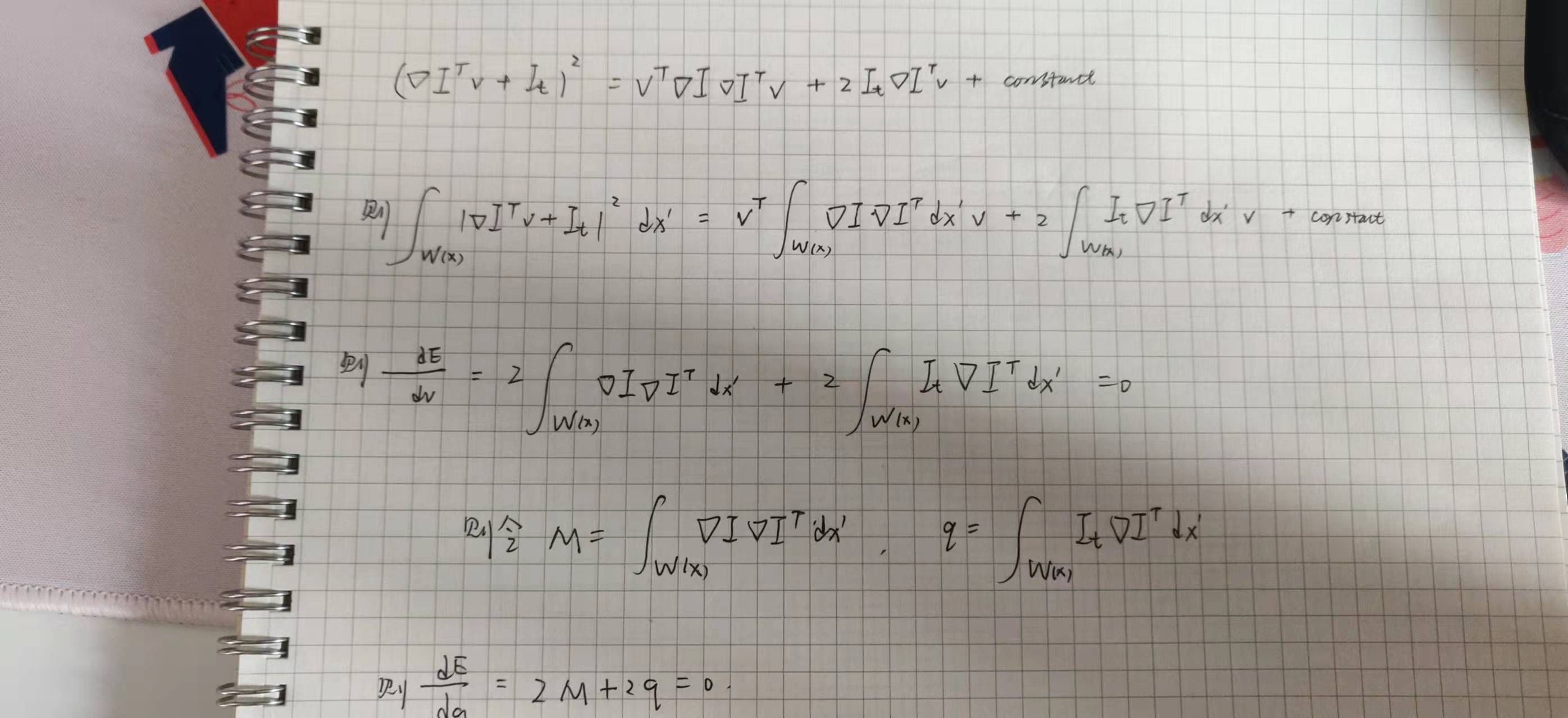
Lucas and Kanade(1981) therefore compute the best velocity vector $v$ for the point $x$ by minimizing the least squares error:
$$
E(v) = \int_{W(x)}|\nabla I(x’, t)^Tv + I_t(x’, t)|^2dx’.
$$

Expanding the terms and setting the derivative to zero one obtains:
$$
\frac{dE}{dv} = 2Mv + 2q = 0,
$$
with
$$
M = \int_{W(x)}\nabla I\nabla I^T dx’, \quad and \quad q = \int_{W(x)}I_t\nabla Idx’.
$$

If $M$ is invertible, i.e. $det(M)\neq 0$, then the solution is:
$$
v = -M^{-1}q.
$$

4.9 Estimating Local Displacements

Translational motion: Lucas & Kanade 1981:
$$
E(b) = \int_{W(x)} |\nabla I^T b+ I_t|^2dx’ \rightarrow min.\\
\frac{dE}{db}=0 \Leftrightarrow b = …
$$
Affine motion: (为window内的像素细致的估计各自的运动)
$$
E(p) = \int_{W(x)} |\nabla I^T S(x’)p+ I_t|^2dx’ \rightarrow min.\\
\frac{dE}{dp}=0 \Leftrightarrow p = …
$$
where:
$$
u(x) = S(x)p = \left(\begin{matrix}
x &y&1&0&0&0\\
0&0&0&x&y&1
\end{matrix}\right)(p_1, p_2, p_3,p_4,p_5,p_6)^T =
\left(\begin{matrix}
p_1x+p_2y+p_3\\
p_4x+p_5y+p_6
\end{matrix}\right).
$$

4.10 When can Small Motion be Estimated?

In the formalism of Lucas and Kanade, one cannot always estimate a translational motion. This problem is often referred to as the aperture problem. It arises for example, if the region in the window $W(x)$ around the point $x$ has entirely constant intensity (for example a white wall), because then $\nabla I(x)=0$ and $I_t(x)=0$ for all points in the window.

In order for the solution of $b$ to be unique the structure tensor:
$$
M(x) = \int_{W(x)} \left(\begin{matrix}
I_x^2 &I_xI_y\\
I_xI_y &I_y^2
\end{matrix} \right)dx’.
$$
needs to be invertible. That means that we must have $det(M)\neq 0$.

If the structure tensor is not invertible but not zero, then one can estimate the normal motion, i.e. the motion in direction of the image gradient.

For those points with $det(M(x))\neq 0$, we can compute a motion vector $b(x)$. This leads to the following simple feature tracker.

4.11 A Simple Feature Tracking Algorithm

Feature tracking over a sequence of images can now be done as follows:

For a given time instance $t$, compute at each point $x\in \Omega$ the structure tensor”
$$
M(x) = \int_{W(x)} \left(\begin{matrix}
I_x^2 &I_xI_y\\
I_xI_y &I_y^2
\end{matrix} \right)dx’.
$$
Mark all points $x\in \Omega$ for which the determinant of $M$ is larger than a threshold $\theta >0$:
$$det(M(x))\geq 0
$$
For all these points the local velocity is given by:
$$
b(x, t) = -M(x)^{-1}\left(\begin{matrix}
\int I_xI_t dx’\\
\int I_yI_t dx’
\end{matrix} \right).
$$
Repeat the above steps for the points $x+b$ at time $t+1$.

4.12 Robust Feature Point Extraction

Even $det(M(x))\neq 0$ does not guarantee robust estimates of velocity—the inverse of $M(x)$ may not be very stable if, for example, the determinant of $M$ is very small. Thus locations with $det(M)\neq 0$ are not always reliable features for tracking.

One of the classical feature detectors was proposed independently by Forstner 1984 and Harris & Stephens 1988.
It is based on the structure tensor:
$$
M(x) = G_{\sigma}*\nabla I \nabla I^T = \int G_\sigma (x-x’)\left(\begin{matrix}
I_x^2 &I_xI_y\\
I_xI_y &I_y^2
\end{matrix} \right)(x’)dx’,
$$
where rather than simple summing over the window $W(x)$ we perform a summation weighted by a Gaussian $G$ of width $\sigma$.
The Forstner/Harris detector is given by:
$$
C(x) = det(M) + \kappa trace^2(M).
$$

One selects points for which $C(x)>\theta$ with a threshold $\theta > 0$.

4.13 Wide Baseline Matching

Corresponding points and regions may look very different in different views. Determining correspondence is a challenge.

In the case of wide baseline matching, large parts of the image plane will not matching at all because they are not visible in the other image. In other words, while a given point may have many potential matches, quite possibly it does not have a correpsonding point in the other image.

4.14 Extensions to Larger Baseline

One of the limitations of tracking features frame by frame is that small errors in the motion accumulate over time and the window gradually moves away from the point that was originally tracked. This is known as drift.
A remedy is to match a given point back to the first frame. This generally implies larger displacements between frames.

Two aspects matter when extending the above simple feature tracking method to somewhat larger displacements:

Since the motion of window between frames is (in general) no longer translational, one needs to generalize the motion model for the window $W(x)$, for example by using an affine motion model.
Since the illumination will change over time (especially when comparing more distant frames), one can replace the sum-of-squared-differences by the normlized cross correlation which is more robost to illumination changes.

4.15 Normlized Cross Correlation （就是用均值和方差进行归一化处理）

The normalized cross correlation is defined as:
$$
NCC(h) = \frac{\int_{W(x)}(I_1(x’)-\bar{I_1})(I_2(h(x’)) - \bar{I_2})dx’}{\sqrt{\int_{W(x)}(I_1(x’)-\bar{I_1})^2dx’ \int_{W(x)}(I_2(h(x’)) - \bar{I_2})^2dx’}}
$$
where $\bar{I_1}$ and $\bar{I_2}$ are the average intensity over the window $W(x)$. By subtracting this average intensity, the measure becomes invariant to additive intensity changes $I\rightarrow I+\gamma$. (对加法不敏感，即均值处理)
Dividing by the intensity variances of each window makes the measure invariant to multiplicative changes $I\rightarrow \gamma I$.(对乘法不敏感，即单位化)
If we stack the normlized intensity values of respective windows into one vector, $v_i\equiv vec(I_i - \bar{I_i})$, then the normlized cross correction is the cosine of the angle between them:
$$
NCC(h) = \cos \angle(v_1, v_2).
$$

4.16 Special Case: Optimal Affine Transformation

The normalized cross correlation can be used to determine the optimal affine transformation between two given patches. Since the affine transformation is given by:
$$
h(x) = Ax + d,
$$
we need to maximize the cross correlation with respect to the 2x2-matrix $A$ and the displacement $d$:
$$
\hat{A}, \hat{d} = \\argmax_{A, d}NCC(A, d).
$$
where
$$
NCC(A, d) = \frac{\int_{W(x)}(I_1(x’)-\bar{I_1})(I_2(Ax’+d) - \bar{I_2})dx’}{\sqrt{\int_{W(x)}(I_1(x’)-\bar{I_1})^2dx’ \int_{W(x)}(I_2(Ax’+d) - \bar{I_2})^2dx’}}
$$
Efficiently finding appropriate optima, however, is a challenge.