多视图几何(五)
Chapter5 Reconstruction from Two Views
5.1. Problem Formulation
In the last sections, we discussed how to identify point correspondences between two consecutive frames. In this section, we will trackle the next next problem, namely that of reconstructing the 3D geometry of cameras and points.
To this end, we will make the following assumptions:
- We assume that we are given a
set of corresponding pointsin two frames taken with the same camera from different vantage points. - We assume that
the scene is static, i.e. none of the observed 3D points moved during the camera motion. - We also assume that the
intrinsic camera (calibration) parameter are known.
We will first estimate the camera motion from the set of corresponding points. Once we know the relative location and orientation of the cameras, we can reconstruct the 3D location of all corresponding points by triangulation.
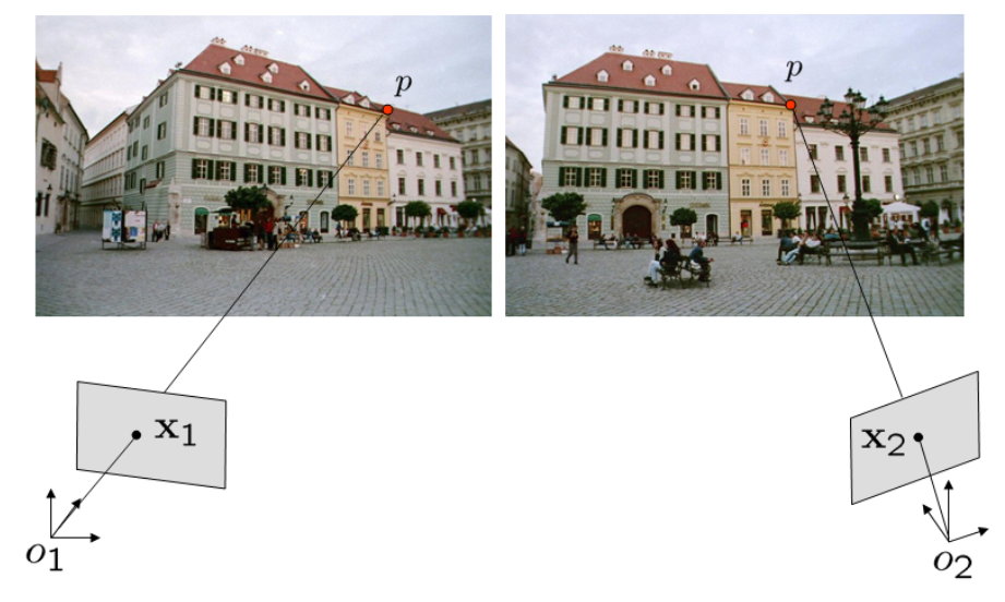
Goal: Estimate camera motion and 3D scene structure from two views.
5.2 The Reconstruction Problem
In general 3D reconstruction is a challenging problem. If we are given two views with 100 feature points in each of them, then we have 200 point coordinates in 2D. The goal is to estimate
- 6 parameters modeling the camera motion $R, T$ and
- $100\times 3$ coordinates for the 3D points $X_j$.
This could be done by minimizing the projection error:
$$
E(R, T, X_1, …,X_{100}) = \sum_j||x_1^j - \pi(X_j)||^2 + ||x_2^j-\pi(R, T, X_j)||^2.
$$
This amounts to a difficult optimization problem called bundle adjustment.
Before we look into this problem, we will first study an elegant solution to entirely get rid of the 3D point coordinates. It leads to the well-known 8-point algorithm.
5.3 Epipolar Geometry: Some Notation
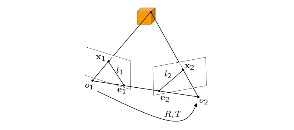
The projections of a point $X$ onto the two images are denoted by $x_1$ and $x_2$. The optical centers of each camera are denoted by $o_1$ and $o_2$. The intersections of the line $(o_1, o_2)$ with each image plane are called the epipoles $e_1$ and $e_2$. The intersections between the epipolar plane $(o_1, o_2, X)$ and the image planes are called epipolar lines $l_1$ and $l_2$. There is one epipolar plane for each 3D point $X$.
5.4 The Epipolar Constraint
We know that $x_1$ (in homogeneous coordinates) is the projection of a 3D point $X$. Given known camera parameters $(K=1)$ and no rotation or translation of the first camera, we merrly have a projection with unknown depth $\lambda_1$. From the first to the second frame we additionally have a camera rotation $R$ and a translation $T$ followed by a projection. This gives the equations:
$$
\lambda_1 x_1 = X, \quad \lambda_2 x_2 = RX+T.
$$
Inserting the first equation into the second, we get:
$$
\lambda_2 x_2 = R(\lambda_1 x_1) + T.
$$
Now we remove the translation by multiplying with $\hat{T}$ $(\hat{T}v \equiv T\times v)$:(两边同时乘以$\hat{T}$这个反对称矩阵,而$\hat{T}T$相当于向量$T$自己和自己做叉乘,即为0向量,这样一来,就可以把上式中的加法去掉)
$$
\lambda_2 \hat{T}x_2 = \lambda_1 \hat{T}Rx_1
$$
And projection onto $x_2$ gives the epipolar constraint:(把两边的向量都投影到$x_2$方向上时,即两边的向量同时和$x_2$向量做内积,也就是两边同时乘以向量$x_2^T$,那左边的向量$\hat{T}x_2=T\times x_2$本身与$x_2$正交,故内积为标量0,而右边就只剩下$\lambda_1 x_2^T\hat{T}Rx_1$,进而$\lambda_1 \neq 0$表示我们观察的3D物体点不在相机的光心处,所以可以把$\lambda_1$约去,最终就剩下了下面的式子:)
$$
x_2^T \hat{T}Rx_1 = 0 \quad( x_1 和x_2都是2D坐标的齐次形式(x,y,1))
$$
The epipolar constraint:
$$
x_2^T \hat{T}Rx_1 = 0
$$
provides a relation between the 2D point coordinates of a 3D point in each of the two images and the camera transformation parameters. The original 3D point coordinates have been removed. The matrix:
$$
E = \hat{T}R \in \mathbb{R}^{3\times 3}
$$
is called the essential matrix. The epipolar constraint is also known as essential constraint or bilinear constraint. Geometrically, this constraint states that the three vectors $\overrightarrow{o_1 X}$, $\overrightarrow{o_2o_1}$ and $\overrightarrow{o_2X}$ form a plane, i.e. the triple product of those vectors (measuring the volume of the parallelpiped) is zero: In coordinates of the second frame $Rx_1$ gives the direction of the vector $\overrightarrow{o_1X}$; $T$ gives the direction of $\overrightarrow{o_2o_1}$, and $x_2$ is proportional to the vector $\overrightarrow{o_2X}$ such that:
$$
volume = x_2^T (T\times Rx_1) = 0
$$
5.5 Properties of the Essential Matrix E
The space of all essential matrices is called the essential space:
$$
\varepsilon \equiv \{\hat{T}R | R\in SO(3), T\in \mathbb{R}^3\} \subset \mathbb{R}^{3\times 3}
$$Theorem [Huang & Faugeras, 1989] (Characterization of the essential matrix) A nonzero matrix $E\in \mathbb{R}^{3\times 3}$ is an essential matrix if and only if $E$ has a singular value decomposition (SVD)$E = U\Sigma V^T$ with:
$$
\Sigma = diag\{\sigma, \sigma, 0\}
$$
for some $\sigma > 0$ and $U, V \in SO(3)$.
Theorem (Pose recovery from the essential matrix): There exist exactly two relative poses $(R, T)$ with $R\in SO(3)$ and $T\in \mathbb{R}^3$ corresponding to an essential matrix $E\in \varepsilon$. For $E=U\Sigma V^T$ we have:
$$
(\hat{T_1}, R_1) = (UR_Z(+\frac{\pi}{2})\Sigma U^T, UR_Z(+\frac{\pi}{2})\Sigma V^T), \
$$
$$
(\hat{T_2}, R_2) = (UR_Z(-\frac{\pi}{2})\Sigma U^T, UR_Z(-\frac{\pi}{2})\Sigma V^T).
$$
(式中我们定义的$R_Z(\theta)=\left(\begin{matrix}
cos(\theta) &-sin(\theta) &0 \\
sin(\theta) &cos(\theta) &0\\
0 &0 & 0
\end{matrix}\right)$, 所以
$R_Z(+\frac{\pi}{2})=\left(\begin{matrix}
0 & -1 &0 \\
1 &0 &0\\
0 &0 & 0
\end{matrix}\right)$, $R_Z(-\frac{\pi}{2})=\left(\begin{matrix}
0 & 1 &0 \\
-1 &0 &0\\
0 &0 & 0
\end{matrix}\right)$)
In general, only one of these gives meaningful (positive) depth values.
5.6 A Basic Reconstruction Algorithm
We have seen that the 2D-coordinates of each 3D point are coupled to the camera parameters $R$ and $T$ through an epipolar constraint. In the following, we will derive a 3D reconstruction algorithm which proceeds as follows:
Recover the essential matrix$E$ from the epipolar constraints associated with a set of point pairs.Extract the relative translation and rotationfrom the essential matrix $E$. (本质矩阵的前两个特征值相等,且第三个特征值为0)
In general, the matrix $E recovered from a set of epipolar constrains will not be an essential matrix. One can resolve this problem in two ways:
- Recover some matrix $E\in\mathbb{R}^{3\times 3}$ from the epipolar constraints and then project it onto the essential space.
- Optimize the epipolar constraints in the essential space.
While the second approach is in principle more accurate it involves a nonlinear constrained optimization. So we will pursue the first approach which is simpler and faster.
5.7 The Eight-Point Linear Algorithm
First we rewrite the epipolar constrainr as a scalar product in the elements of the matrix $E$ and the coordinates of the points $\textbf{x}_1 $ and $\textbf{x}_2$. Let
$$
E^s = (\theta_{11}, \theta_{21}, \theta_{31},
\theta_{12}, \theta_{22}, \theta_{32},
\theta_{13}, \theta_{23}, \theta_{33})^T \in \mathbb{R}^9
$$
be the vector of elements of $E$ and
$$
a = \textbf{x}_1 \otimes \textbf{x}_2
$$
the Kronecker product of the vectors $\textbf{x}_i = (x_i, y_i, z_i)$, defined as $a = (x_1x_2, x_1y_2, x_1z_2, y_1x_2, y_1y_2, y_1z_2, z_1x_2, z_1y_2, z_1z_2)^T \in \mathbb{R}^9$.
Then the epipolar constraint can be written as:
$$
\textbf{x}_2^TE\textbf{x}_1 = a^TE^s = 0.
$$
For $n$ point pairs, we can combine this into the linear system:
$$
\chi E^s = 0, \quad \chi = (a^1, a^2, …, a^n)^T.
$$
According to
$$
\chi E^s = 0, \quad with \chi = (a^1,a^2, …, a^n)^T.
$$
we see that the vector of coefficients of the essential matrix $E$ defines the null space of the matrix $\chi$. In order for the abover system to have a unique solution (up to a scaling factor and ruling out the trivial solution $E=0$), the rank of the matrix $\chi$ needs to be exactly 8. Therefore we need at least 8 point pairs.
In certain degenerate cases, the solution for the essential matrix is not unique even if we have 8 or more point pairs. One such example is the case that all points lie on the a line or on a plane.
Clearly, we will not be able to recover the sign of $E$. Since with each $E$, there are two possible assignments of rotation $R$ and translation $T$, we therefore end up with four possible solutions for rotation and translation.
5.8 Projection onto Essential Space
The numerically estimated coefficients $E^s$ will in general not correspond to an essential matrix. One can resolve this problem by projecting it back to the essential space:

Theorem (Projection onto essential space): Let $F \in \mathbb{R}^{3\times 3}$ be an arbitrary matrix with SVD
$F = Udiag{\lambda_1, \lambda_2, \lambda_3}V^T, \lambda_1\geq \lambda_2\geq \lambda_3$. Then the essential matrix $E$ which minimizes the Frobenius norm $||F-E||^2_t$ is given by:
$$
E = Udiag{\sigma ,\sigma, 0 }V^T, \quad with \ \sigma=\frac{\lambda_1 + \lambda_2}{2}.
$$
5.9 Eight Point Algorithm (Longuet-Higgins 1981)
Given a set of $n=8$ or more point pairs $\textbf{x}_1^i$, $\textbf{x}_2^i$:
Compute an approximation of the essential matrix.Construct the matrix $\chi = (a^1, a^2, …, a^n)^T$, where $a^i = \textbf{x}1^i \otimes \textbf{x}2^i$. Find the vector $E^s\in \mathbb{R}^9$ which minimizes $||\chi E^s||$ as the ninth column of $V{\chi}$ in the SVD $\chi =U{\chi}\Sigma_{\chi}V^T_{\chi}$. Unstack $E^s$ into $3\times 3$-matrix $E$.Project onto essential space. Compute the SVD $E=Udiag{\sigma_1, \sigma_2, \sigma_3}V^T$. Since in the reconstruction, $E$ is only defined up to a scalar, we project $E$ onto thenormlized essential spaceby replacing the singular values $\sigma_1, \sigma_2, \sigma_3$ with 1, 1, 0.Recover the displacement from the essential matrix. The four possible solutions for rotation and translation are:$$
R = UR_Z^T(\pm \frac{\pi}{2})V^T, \quad \hat{T} = UR_Z(\pm \frac{\pi}{2})\Sigma U^T,
$$with a rotation by $\pm \frac{\pi}{2}$ around $z$:
$$
R_Z^T(\pm \frac{\pi}{2}) = \left(\begin{matrix}
0 &\pm 1 & 0 \\
\mp 1 & 0 & 0 \\
0 & 0 & 1
\end{matrix} \right).
$$
5.10 Do we need Eight Points? (用5点法也可求解)
The above reasoning showed that we need at least eight points in order for the matrix $\chi$ to have rank 8 and therefore guarantee a unique solution for $E$. Yet, one can take into account the special structure of $E$. The space of essential matrices is actually a five dimensional space, i.e. $E$ only has 5 (and not 9) degrees of freedom.
A simple way to take into account the algebraic properties of $E$ is to make use of the fact that $det(E)=0$. If now we have only 7 point pairs, the null space of $\chi$ will have (at least) Dimension 2, spanned by two vectors $E_1$ and $E_2$. Then we can solve for $E$ by determining $\alpha$ such that:
$$
det(E) = det(E_1 + \alpha E_2) = 0.
$$
Along similar lines, Kruppa proved in 1913 that one needs only five point pairs to recover $(R, T)$. In the case of degenerate motion (for example planar or circular motion), one can resolve the problem with even fewer point pairs.
5.11 Limitations and Further Extensions
Among the four possible solutions for $R$ and $T$, there is generally only one meaningful one (which assigns positive depth to all points).
The algorithm fairs if the translation is exactly 0, since then $E=0$ and nothing can be recovered. Due to noise this typically does not happen.
In the case of infiitesimal view point change, one can adapt the eight point algorithm to the continuous motion case, where the epipolar constraint is replaced by the continuous epipolar constraint. Rather than recovering $(R, T)$ one recovers the linear and angular velocity of the camera.
In the case of independently moving objects, one can generalize the epipolar constraint. For two motions for example we have:
$$
(x_2^TE_1x_1)(x_2^TE_2x_1) = 0
$$
with two essential matrices $E_1$ and $E_2$. Given a sufficiently large number of point pairs, one can solve the respective equations for multiple essential matrices using polynomial factorization.
5.12 Structure Reconstruction
The linear eight-point algorithm allowed us to estimate the camera transformation parameters $R$ and $T$ from a set of corresponding point pairs. Yet, the essential matrix $E$ and hence the translation $T$ are only defined up to an arbitrary scale $\gamma \in \mathbb{R}^{+}$, with $||E||=||T||=1$. After recovering $R$ and $T$, we therefore have for point $X^j$:
$$
\lambda_2^j \textbf{x}_2^j = \lambda_1^j R\textbf{x}_1^j + \gamma T, \quad j=1, …, n,
$$
with unknown scale parameters $\lambda_i^j$. We can eliminate one of these scales by applying $\widehat{\textbf{x}_2^j}$:
$$
\lambda_1^j \widehat{\textbf{x}_2^j}R\textbf{x}_1^j + \gamma\widehat{\textbf{x}_2^j}T = 0, \quad j=1,…,n.
$$
This corresponds to $n$ linear systems of the form:
$$
(\widehat{\textbf{x}_2^j}R\textbf{x}_1^j, \widehat{\textbf{x}_2^j}T)\left(\begin{matrix}
\lambda_1^j \\
\gamma
\end{matrix}\right) = 0, \quad j=1,…,n.
$$
Combining the parameters $\vec{\lambda}=(\lambda_1^1, \lambda_1^2,…,\lambda_1^n, \gamma)^T\in \mathbb{R}^{n+1}$, we get the linear equation system
$$
M\vec{\lambda} = 0
$$
with
$$
M \equiv \left(\begin{matrix}
\widehat{\textbf{x}_2^1}R\textbf{x}_1^1 &0 & 0& 0 & 0 & \widehat{\textbf{x}_2^1}T\\
0 &\widehat{\textbf{x}_2^2}R\textbf{x}_1^2 & 0& 0 & 0 & \widehat{\textbf{x}_2^2}T\\
0 & 0 &\ddots &0 & 0 &\vdots \\
0 &0 & 0& \widehat{\textbf{x}_2^{n-1}}R\textbf{x}_1^{n-1} & 0 & \widehat{\textbf{x}_2^{n-1}}T\\
0 & 0 & 0& 0 & \widehat{\textbf{x}_2^n}R\textbf{x}_1^n & \widehat{\textbf{x}_2^n}T\\
\end{matrix}\right)
$$
(求解的优化问题是:
$$
\min_{\vec{\lambda}} ||M\vec{\lambda}||^2 = \min_{\vec{\lambda}}\lambda^TM^TM\lambda, \quad ||\lambda||=1.
$$
Note: 进一步,我们让优化目标函数对$\vec{\lambda}$求导数,导数最小处就是$\vec{\lambda}$的解。令导数为0有: $2M^TM\vec{\lambda}=0$,进一步,由于矩阵可以通过其特征值进行等价代换,即著名的$Ax=\lambda x$中,一个矩阵$A$乘以他的一个特征向量$x$等于该特征向量对应的特征值$\lambda$与该特征向量$x$的乘积,因此可以将上面的导数$2M^TM\vec{\lambda}=0$进行变换,假设矩阵$M^TM$的一个最小的一个接近于0的特征值是$\eta$,且该特征值对应的特征向量为$p$,即$M^TM p = \eta p$,那么上面的导数就可以被估计成$2M^TMp = \eta p \approx 0$,也就是说,原来优化问题的解$\vec{\lambda}$近似是矩阵$M^TM$的最小特征值对应的特征向量,求解完毕。 )
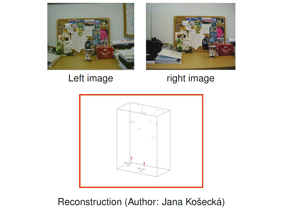
The linear least squares estimate for $\vec{\lambda}$ is given by the eigenvector corresponding to the smallest eigenvalue of $M^TM$. It is only defined up to a global scale. It reflects the ambiguity that the camera has moved twice the distance, the scane is twice larger and twice as far away.
5.13 Example
5.14 Optimality in Noisy Real World Conditions
The eight-point algorithm discussed before has several nice properties. In particular, we found closed-form solutions to estimate the camera parameters and the 3D structure, based on singular value decomposition. However, if we have noisy data ${\tilde{\textbf{x}_1}}$, ${\tilde{\textbf{x}}_2}$ (correspondences not exact or even incorrect), then we have:
- no quarantee that $R$ and $T$ are as close as possible to the true solution.
- no guarantee that we will get a consistent reconstruction.
5.15 Nonlinear Optimization Methods
In order to take noise and statistical fluctutation into account, one can revert to a Bayesian formulation and determine the most likely camera transformlation $R, T$ and ‘true’ 2D coordinates $\textbf{x}$ given the measured coordinates $\tilde{\textbf{x}}$, by performing a maximum a posteriori estimate:
$$
\\argmax_{\textbf{x}, R, T}\mathcal{P}(\textbf{x}, R, T|{\tilde{\textbf{x}}})=\\argmax_{\textbf{x}, R, T}\mathcal{P}(\tilde{\textbf{x}}|\textbf{x}, R, T)\mathcal{P}(\textbf{x}, R, T)
$$
This approach will however involve modeling probability densities $\mathcal{P}$ on the fairly complicated space $SO(3)\times \mathbb{S}^2$ of rotation and translation parameters, as $R\in SO(3)$ and $T\in \mathbb{S}^2$ (3D translation with unit length).
Alternatively, one can perform a constrained optimization by minimizing a cost function (similarity to measurements):
$$
\phi(\textbf{x}, R, T) = \sum_{j=1}^n \sum_{i=1}^2 ||\tilde{\textbf{x}_i^j}-\textbf{x}_i^j||^2
$$
suject to (consistent geometry):
$$
\textbf{x}_2^{jT}\hat{T}R\textbf{x}_1^j = 0, \quad \textbf{x}_1^{jT}e_3=1, \quad \textbf{x}_2^{jT}e_3 = 1, j=1,2,…,n. (where \ e_3=(0,0,1))
$$
5.16 Bundle Adjustment
Interestingly, the unknown depth parameters $\lambda_i$ do not actually appear in the above cost functions.
The depth parameters appear directly in the unconstrained optimization problem:
$$
\sum_{j=1}^n ||{\textbf{x}_1^j}-\pi_1(\textbf{X}{^j})||^2 + ||\tilde{\textbf{x}_2^j}-\pi_2(\textbf{X}{^j})||^2,
$$
where $\pi_i$denotes the projections onto the two images. Expressed in coordinates of the first camera frame, this is equal to the cost function:
$$
\phi(\textbf{x}1, R, T, \lambda) = \sum{j=1}^n ||\tilde{\textbf{x}_1^j}-\textbf{x}_1^j||^2 + ||\tilde{\textbf{x}_2^j} - \pi(R\lambda_1^j\textbf{x}_1^j+T)||^2.
$$
This optimization procedure is known as bundle adjustment. The constrained optimization and the unconstrained bundle adjustment can be seen as different parameterizations of the same optimization objective.
5.17 Degenerate Configurations
The eight-point algorithm only provides unique solutions (up to a scalar factor) if all 3D points are in a “general position”. This is no longer the case for certain degenerate configurations, for which all points lie on certain 2D surfaces which are called critical surfaces.
While most critical configurations do not actually arise in practice, a specific degenerate configuration which does arise often is the case that all points lie on 2 2D plane (such as floors, table, walls,…).
For the structure-from-motion problem in the context of points on a plane, one can exploit additional constraints which leads to the so-called four-point algorithm.
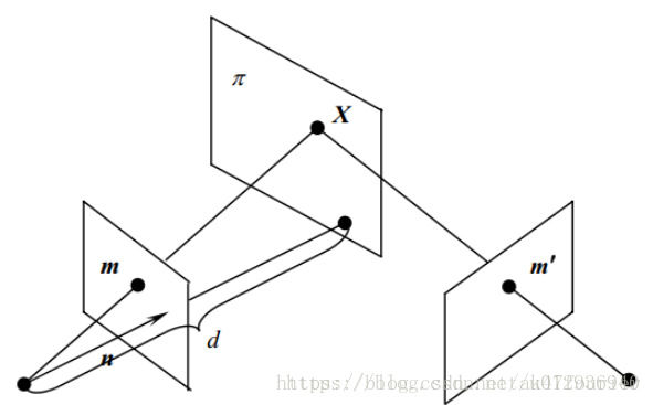
5.18 Planar Homographies
Let us assume that all points lie on a plane. If $\textbf{X}_1\in\mathbb{R}^3$ denotes the point coordinates in the first frame, and these lie on a plane with normal vector $N\in \mathbb{S}^2$, then we have:
$$
N^T\textbf{X}_1 = d \Leftrightarrow\frac{1}{d}N^T\textbf{X}_1 = 1.
$$
In frame two, we therefore have the coordinates:
$$
\textbf{X}_2=R\textbf{X}_1 +T = R\textbf{X}_1 + T\frac{1}{d}N^T\textbf{X}_1 = (R+\frac{1}{d}TN^T)\textbf{X}_1 \equiv H\textbf{X}_1,
$$
where
$$
H = R + \frac{1}{d}TN^T \in \mathbb{R}^{3\times 3}
$$
is called a homography matrix. Inserting the 2D coordinates, we get:
$$
\lambda_2 \textbf{x}_2 = H\lambda_1\textbf{x}_1 \Leftrightarrow\textbf{x}_2\sim H\textbf{x}_1.
$$
where $\sim$ means equality up to scaling. This expression is called a planar homography. $H$ depends on camera and plane parameters.
5.19 From Point Pairs to Homography
For a pair of corresponding 2D points we therefore have:
$$
\lambda_2 \textbf{x}_2 = H\lambda_1 \textbf{x}_1.
$$
By multiplying with $\widehat{\textbf{x}_2}$ we can eliminate $\lambda_2$ and obtain:
$$
\widehat{\textbf{x}_2}H\textbf{x}_1 = 0
$$
This equation is called the planar epipolar constraint or planar homography constraint.
Again, we can cast this equation into the form:
$$
\textbf{a}^TH^s = \vec{0} \in \mathbb{R}^{3\times 1}
$$
where we have stacked the elements of $H$ into a vector:
$$
H^s = (H_{11}, H_{21}, …, H_{33})\in \mathbb{R}^9,
$$
and introduced the matrix:
$$
\textbf{a} \equiv \textbf{x}_1 \otimes \widehat{\textbf{x}_2} \in \mathbb{R}^{9\times 3}
$$
(原因在于$\widehat{\textbf{x}_2}$是一个$3\times 3$的矩阵,所以得到的克罗内克乘积是一个$9\times 3$的矩阵,而不是$9\times 1$的矩阵。所以$\textbf{a}^TH^s = \vec{0} \in \mathbb{R}^{3\times 1}$会提供给我们3个方程,但不幸的是其中只有两个方程独立,即rank=2,因为反对称矩阵$\widehat{\textbf{x}_2}$的性质不好,其秩为2.这样下来,一对点就可以提供两个方程,此前为了估计本质矩阵,general的情况下我们需要8对点,那么现在估计单应矩阵时,general情况下我们就只需要4对点了。)
5.20 The Four Point Algorithm
Let us now assume we have $n\geq 4$ pairs of corresponding 2D points ${\textbf{x}_1^j, \textbf{x}_2^j}, j=1,…,n$ in the two images. Each point pair induces a matrix $\textbf{a}^j$, we integrate these into a larger matrix:
$$
\chi \equiv (\textbf{a}^1, …, \textbf{a}^n)^T \in \mathbb{R}^{3n\times 9},
$$
and obtain the system:
$$
\chi H^s = \vec{0} \in \mathbb{R}^{3n \times 1}
$$
As in the case of the essential matrix, the homography matrix can be estimated up to a scale factor.
This gives rise to the four point algorithm:
- For the point pairs, compute the matrix $\chi$.
- Compute a solution $H^s$ for the above equation by singular value decomposition of $\chi$.
- Extract the motion parameters from the homography matrix $H = R + \frac{1}{d}TN^T$.(这一步中从单应矩阵$H$中恢复相机的运动$R,T$比较麻烦,但是有方法的。)
5.21 General Comment
Clearly, the derivation of the four-point algorithm is in close analogy to that of the eight-point algorithm.
Rather than estimating the essential matrix $E$ one estimates the homography matrix $H$ to derive $R$ and $T$. In the four-point algorithm, the homography matrix is decomposed into $R, N$ and $T/d$. In other words, one can reconstruct the normal of the plane, but the translation is only obtained in units of the offset $d$ of the plane and the origin.
The 3D structure of the points can then be computed in the same manner as before.
Since one uses the strong constraint that all points lie in a plane, the four-point algorithm only requires four correspondences.
There exist numerous relations between the essential matrix $E=\hat{T}R$ and the corresponding homography matrix $H=R+Tu^T$ with some $u\in \mathbb{R}^3$, in particular:
$$
E = \hat{T}H, \quad H^TE + E^TH = 0.
$$
5.22 The Case of an Uncalibrated Camera
The reconstruction algorithms introduced above all assume that the camera is calibrated (K=1). The general transformation from a 3D point to the image is given by:
$$
\lambda\textbf{x}’ = K\Pi_0 g\textbf{X} = (KR, KT)\textbf{X},
$$
with the intrinsic parameter matrix or calibration matrix:
$$
K = \left(\begin{matrix}
fs_x &s_\theta & o_x\\
0 &fs_y & o_y\\
0 &0 &1
\end{matrix}\right) \in \mathbb{R}^{3\times 3}.
$$
The calibration matrix maps metric coordinates into image (pixel) coordinates, using the focal length $f$, the optical center $o_x, o_y$, the pixel size $s_x, s_y$ and a skew factor $s_\theta$. If these parameters are known then one can simply transform the pixel coordinates $\textbf{x}’$ to normalized coordinates $\textbf{x} = K^{-1}\textbf{x}’$ to obtain the representation used in the previous sections. This amounts to centering the coordinates with respect to the optical center etc.
5.23 The Fundamental Matrix
If the camera parameter $K$ cannot be estimated in a calibration procedure beforehand, then one has to deal with reconstruction from uncalibrated views.
By transforming all image coordinates $\textbf{x}’$ with the inverse calibration matrix $K^{-1}$ into metric coordinates $\textbf{x}$, we obtain the epipolar constraint for uncalibrated cameras:
$$
\textbf{x}_2^T\hat{T}R\textbf{x}_1 = 0\Leftrightarrow \textbf{x}_2^{‘T}K^{-T}\hat{T}RK^{-1}\textbf{x}_1^{‘} = 0
$$
(推广也比较直观,坐标$x_1, x_2$是在归一化坐标平面中,而坐标$x’_1, x’_2$是在真实的焦平面处,实际中将世界坐标系中的点转换为图像平面的过程中时,归一化坐标平面是在真实的焦平面之前的,故有$x‘_1 = Kx_1, x’_2 = Kx_2$,即$x_1 = K^{-1}x’_1, x_2=K^{-1}x’_2$, 代入到归一化平面中的对极约束中我们就得到了基础矩阵版本的对极约束。)
which can be written as
$$
\textbf{x}_2^{‘T}F\textbf{x’}_1 = 0,
$$
with the fundamental matrix defined as:
$$
F \equiv K^{-T}\hat{T}RK^{-1} = K^{-T}EK^{-1}.
$$
Since the invertible matrix $K$ does not affect the rank of this matrix, we know that $F$ has an SVD $F=U\Sigma V^T$ with $\Sigma = diag(\sigma_1, \sigma_2, 0)$. In fact, any matrix of rank 2 can be a fundamental matrix.
5.24 Limitations (完全从基础矩阵中恢复出相机运动R,T较难实施)
While it is straight-forward to extend the eight-point algorithm, such that one can extract a fundamental matrix from a set of corresponding image points, it is less straight forward how to proceed from there.
Firstly, one cannot impose a strong constraint on the specific structure of the fundamental matrix (apart from the fact that the last singular value is zero).
Secondly, for a given fundamental matrix $F$, there does not exist a finite number of decompositions into extrinsic parameters $R, T$ and intrinsic parameters $K$ (even apart from the global scale factor).
As a consequence, one can only determine so-called projective reconstructions, i.e. reconstructions of geometry and camera position which are defined up to a so-called projective transformation.
As a solution, one typically choses a canonical reconstruction from the family of possible reconstructions.
 wechat
 alipay