多视图几何(三)
Chapter 3 Perspective Projection
3.1 Mathematics of Perspective Projection
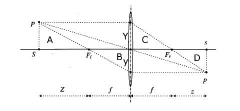
The perspective transformation $\pi$ from a point with coordinates $\textbf{X}=(X,Y,Z)\in \mathbb{R}^3$ relative to the reference frame centered at the optical center and with z-axis being the optical axis (of the lens) is obtained by comparing similar triangles $\textbf{A}$ and $\textbf{B}$:
$$
\frac{Y}{Z} = -\frac{y}{f} \Leftrightarrow y = -f\frac{Y}{Z}.
$$
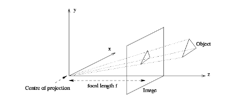
To simplify equations, one flips the signs of x- and y-axes, which amounts to considering the image plane to be in front of the center of projection (rather than behind it). The perspective transformation $\pi$ is therefore given by:
$$
\pi : \mathbb{R}^3 \rightarrow \mathbb{R}^2; \quad \textbf{X}\mapsto x=\pi(\textbf{X})=\left(\begin{matrix} f\frac{X}{Z} \\ f\frac{Y}{Z}\end{matrix}\right).
$$
3.2 An Ideal Perspective Projection
In homogeneous coordinates, the perspective transformation is given by:
$$
Z\textbf{x} = Z\left(\begin{matrix}
x\\y\\1
\end{matrix}\right)=
\left(\begin{matrix}
f & 0&0 &0\\
0 &f &0 &0\\
0 &0&1& 0
\end{matrix}\right)\left(\begin{matrix}
X\\Y\\ Z \\1
\end{matrix}\right) = K_f\Pi_0 \textbf{X},
$$
where we have introduced the two matrices:
$$
K_f \equiv \left(\begin{matrix}
f & 0& 0\\
0 & f &0 \\
0 & 0 & 1
\end{matrix}\right) and\quad \Pi_0 \equiv
\left(\begin{matrix}
1 &0 &0 &0 \\
0 &1 &0 & 0 \\
0 &0 &1 &0
\end{matrix}\right).
$$
The matrix $\Pi_0$ is referred to as the standard projection matrix. Assuming $Z$ to be a constant $\lambda >0$, we obtain:
$$
\lambda x = K_f\Pi_0 \textbf{X}.
$$
From the previous lectures, we know that due to the rigid motion of the camera, the point $\textbf{X}$ in camera coordinates is given as function of the point in world co ordinates $\textbf{X}_0$ by:
$$
\textbf{X} = R\textbf{X}_0 + T,
$$
or in homogeneous coordinates $\textbf{X}=(X, Y, Z, 1)^T$:
$$
\textbf{X} = g\textbf{X}_0 = \left(\begin{matrix}
R &T\\
0 &1
\end{matrix}\right)\textbf{X}_0.
$$
In total, the transformaiton from world coordinates to image coordinates is therefore given by:
$$
\lambda \textbf{x}=K_f\Pi _0 g\textbf{X}_0.
$$
If the focal length $f$ is known, it can be normlized to 1 (by changing the units of the image cooedinates),such that:
$$
\lambda \textbf{x} = \Pi_0 \textbf{X} = \Pi_0 g \textbf{X}_0.
$$
3.3 Intrinsic Camera Parameters
(从世界坐标系—>camera坐标系—>image坐标系—>pixel坐标系)
If the camera is not centered at the optical center, we have an additional translation $o_x, o_y$ and if pixel coordinates do not have unit scale, we need to introduce an additional scaling in x- and y-direction by $s_x$ and $s_y$. If the pixels are not rectangular, we have a skew factor $s_\theta$.
The pixel coordinates $(x’, y’, 1)$ as a function of homogeneous camera coordinates $\textbf{X}$ are then given by:
$$
\lambda \left(\begin{matrix}
x’\\y’\\1
\end{matrix}\right)=\underbrace{\left(\begin{matrix}
s_x &s_y &o_x\\
0 &s_y &o_y \\
0 & 0& 1
\end{matrix}\right)}{\equiv K_s}
\underbrace{\left(\begin{matrix}
f &0&0\\
0 &f&0\\
0 & 0& 1
\end{matrix}\right)}{\equiv K_f}
\underbrace{\left(\begin{matrix}
1&0&0&0\\
0&1&0&0\\
0&0&1&0
\end{matrix}\right)}_{\equiv \Pi_0}
\left(\begin{matrix}
X\\Y\\Z\\1
\end{matrix}\right)
$$
After the perspective projection $\Pi_0$ (with focal length 1), we have an additional transformation which depends on the (intrinsic) camera parameters. This can be expressed by the intrisic parameter matrix $K=K_sK_f$.
3.4 The Intrinsic Parameter Matrix
All intrinsic camera parameter therefore enetr the intrinsic parameter matrix:
$$
K \equiv K_sK_f = \left(\begin{matrix}
fs_x&fs_\theta&o_x\\
0&fs_y&o_y\\
0&0&1
\end{matrix}\right).
$$
As a function of the world coordinates $\textbf{X}_0$, we therefore have:
$$
\lambda \textbf{x}’ = K\Pi_0 \textbf{X} = K\Pi_0 g\textbf{X}_0 \equiv \Pi \textbf{X}_0.
$$
The $3\times 4$ matrix $\Pi\equiv K\Pi_0 g=(KR, KT)$ is called a general projection matrix.
Although the above equation looks like a linear one, we still have the scale parameter $\lambda$. Dividing by $\lambda$ gives:
$$
x’ = \frac{\pi_1^T\textbf{X}_0}{\pi_3^T\textbf{X}_0}, \quad y’=\frac{\pi_2^T\textbf{X}_0}{\pi_3^T\textbf{X}_0}, \quad z’=1,
$$
where $\pi_1^T,\pi_2^T,\pi_3^T \in \mathbb{R}^4$ are the three rows of the projection matrix $\Pi$.
The entries of the intrinsic parameter matrix:
$$
\left(\begin{matrix}
fs_x&fs_\theta&o_x\\
0&fs_y&o_y\\
0&0&1
\end{matrix}\right),
$$
can be interpreted as follows:
$o_x:$ x-coordinate of principal point in pixels,
$o_y$: y-coordinate of principal point in pixels,
$fs_x=\alpha_x$:size of unit length in horizontal pixels,
$fs_y=\alpha_y$:size of unit length in vertical pixels,
$\alpha_x / \alpha_y$: aspect ratio $\sigma$,
$fs_\theta$: skew of pixel, often close to zero.
3.5 Spherical Perspective Projection
The perspective pinhole camera introduced above considers a planar imaging surface. Instead, one can consider a spherical projection surface given by the unit sphere $\mathbb{S}^2\equiv {\textbf{x}\in \mathbb{R}^3 | |\textbf{x}|=1}$. The spherical projection $\pi_s$ of a 3D point $\textbf{X}$ is given by:
$$
\pi_s :\mathbb{R}^3 \rightarrow \mathbb{S}; \quad \textbf{X} \mapsto \textbf{x}=\frac{\textbf{X}}{\textbf{|X|}}.
$$
The pixel coordinates $\textbf{x}’$ as a function of the world coordinates $\textbf{X}_0$ are:
$$
\lambda \textbf{x}’ = K\Pi_0 g\textbf{X}_0,
$$
except that the scalar factor is now $\lambda=|\textbf{X}|=\sqrt{X^2+Y^2+Z^2}$. One often writes $\textbf{x}~\textbf{y}$ for homogeneous vectors $\textbf{x}$ and $\textbf{y}$ if they are equal up to a scalar factor. Then we can write:
$$
\textbf{x}’~\Pi \textbf{X}_0 = K\Pi_0 g\textbf{X}_0.
$$
This property holds for any imaging surface, as long as the ray between $\textbf{X}$ and the origin intersects the imaging surface.
3.6 Radial Distortion
The intrinsic parameters in the matrix $K$ model linear distortions in the transformations to pixel coordinates. In practice, however, one can also encounter significant distortions along the radial axis, in particular if a wide field of view is used or if one uses cheaper cameras such as webcams. A simple effective model for such distortions is:
$$
x = x_d (1+a_1r^2 + a_2r^4), \quad y = y_d(1+a_1r^2+a_2r^4),
$$
where $\textbf{x}_d\equiv (x_d, y_d)$ is the diatorted point, $r^2=x_d^2+y_d^2$. If a calibration rig is available, the distortion parameter $a_1$ and $a_2$ can be estimated.
Alternatively, one can estimate a distortion model directly from the images. A more general model is :
$$
\textbf{x}=c+f(r)(\textbf{x}_d - c), \ with \ f(r)=1+ a_1r + a_2r^2 + a_3r^3 + a_4r^4,
$$
Here, $r = |\textbf{x} -c|$ is the distance to an arbitrary center of distortion $c$ and the distortion correction factor $f(r)$ is an arbitrary 4-th order expression. Parameter are computed from disrtotions of straight lines or simultaneously with the 3D reconstruction.
3.7 Preimage of Points and Lines
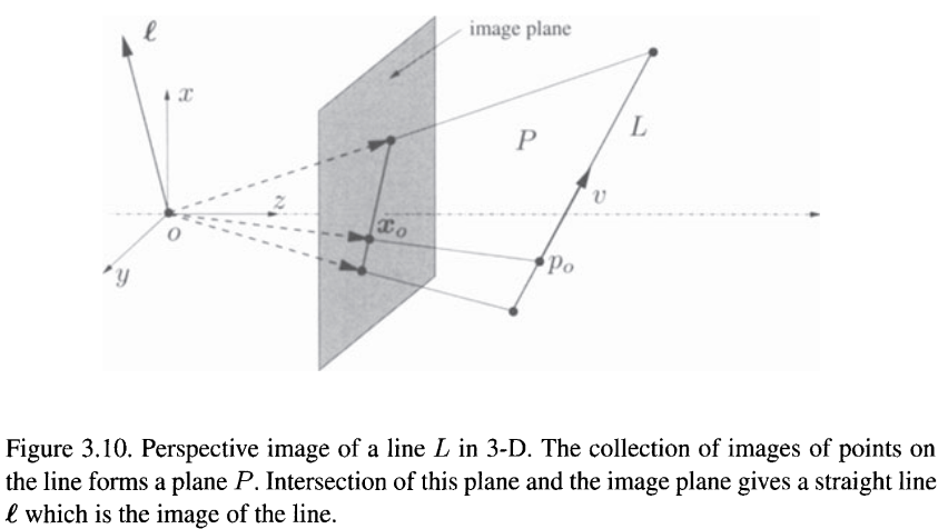
The perspective transformation introduced above allows to define images for arbitrary geometric entities by simply transformaing all points of the entity. However, due to the unknown scale factor, each point is mapped not to a single point $\textbf{x}$, but to an qquivalence class of points $\textbf{y}~\textbf{x}$. It is therefore useful to study how lines are transformed. A line $L$ in 3-D is characterized by a base point $\textbf{X}_0= (X_0, Y_0, Z_0, 1)^T \in \mathbb{R}^4$ and a vector $\textbf{V}=(V_1, V_2, V_3, 0)^T\in \mathbb{R}^4$:
$$
\textbf{X}=\textbf{X}_0 + \mu\textbf{V}, \quad \mu\in\mathbb{R}.
$$
The image of the line $L$ is given by:
$$
\textbf{x}~\Pi_0 \textbf{X} = \Pi_0 (\textbf{X}_0 + \mu \textbf{V}) = \Pi_0 \textbf{X}_0 + \mu \Pi_0 \textbf{V}.
$$
All points $\textbf{x}$ treated as vectors from the origin $o$ span a 2-D subspace $P$. The intersection of this plane $P$ with the image plane gives the image of the line. $P$ is called the preimage of the line.
A preimage of a point or a line in the image plane is the largest set of 3D points that give rise to an image equal to the given point or line.
Preimages can be defined for curves or other more complicated geometric structures. In the case of points and lines, however, the preimage is a subspace of $\mathbb{R}^3$. This subspace can also be represented by its orthogonal complement, i.e. the normal vector in the case of a plane. This complement is called the coimage. The coimage of a point or a line is the subspace in $\mathbb{R}^3$ that is the (unique) orthogonal complement of its preimage. Image, preimage and coimage are equivalent because they uniquely determine one another:
$$
image = preimage \cap image plane, \quad preimage = span(image), \\
$$
$$
preimage = coimage^{\perp}, \quad coimage = preimage^{\perp}.
$$
3.8 Preimage and Colimage of Points and Lines
In the case of the line $L$, the preimage is a 2D subspace, characterized by the 1D colimage given by the span of its normal vector $\ell \in \mathbb{R}^3$. All points of the preimage, and hence all points $\textbf{x}$ of the image of $L$ are orthogonal to $\ell$:
$$
\ell^T\textbf{x} = 0.
$$
The space of all vectors orthogonal to $\ell$ is spanned by the row vectors of $\hat{\ell}$, thus we have:
$$
P = span(\hat{\ell}).
$$
In the case that $\textbf{x}$ is the image of a point $p$, the preimage is a line and the colimage is the plane orthogonal to $\textbf{x}$, i.e. it is spanned by the rows of the matrix $\hat{x}$.
In summary we have the following table:
| Image | Preimage | Colimage | |
|---|---|---|---|
| Point | span($\textbf{x}$)$\cap$ im.plane | span($\textbf{x}$)$\subset\mathbb{R}^3$ | span($\textbf{x}$)$\subset\mathbb{R}^3$ |
| Line | span($\hat{\ell}$)$\cap$ im.plane | span($\hat{\ell}$)$\subset\mathbb{R}^3$ | span($\hat{\ell}$)$\subset\mathbb{R}^3$ |
3.9 Summary
In this part of the lecture, we studied the perspective projection which takes us from the 3D (4D) camera coordinates to 2D camera image coordinates and pixel coordinates. In homogeneous coordinates, we have the transformations:
$$
4D\ Wolrd\ coordinates \stackrel{g\in SE(3)}\longrightarrow 4D \ {Camera \ coordinates} \stackrel{K_f\Pi_0}{\longrightarrow} 3D \ {image \ coordinates}\stackrel{K_s}{\longrightarrow} 3D \ {pixel \ coordinates} (齐次坐标形式).
$$
In particular, we can summarize the (intrinsic) camera parameters in the matrix:
$$
K = K_sK_f.
$$
The full transformation from world coordinates $\textbf{X}_0$ to pixel coordinates $\textbf{x}’$ is given by :
$$
\lambda \textbf{x}’ = K\Pi_0 g\textbf{X}_0.
$$
Moreover, for the images of points and lines we introduced the notions of preimage (maximal point set which is consistent with a given image) and colimage (its orthogonal complement). Both can be used equivlently to the image.
3.10 Projective Geometry
In order to formally write transformation by linear operations, we made extensive use of homogenoeus coordinates to represent a 3D point as a 4D-vector $(X,Y,Z,1)$ with the last coordinate fixed to 1. This normlization is not always necessary: One can represent 3D points by a general 4D vector:
$$
\textbf{X} = (XW, YW, ZW, W)\in \mathbb{R}^4,
$$
remembering that merely the direction of this vector is of importance. We therefore identify the point in homogeneous coordinates with the line connecting it with the origin. This leads to the definition of projective coordinates.
An n-dimensional projective space $\mathbb{P}^n$ is the set of all one-dimensional subspaces (i.e. lines through the origin) of the vector space $\mathbb{R}^{n+1}$. A point $p\in \mathbb{P}^n$ can then be assigned homogeneous coordinates $\textbf{X}=(x_1, …, x_{n+1})^T$, among which at least one $x$ is nonzero. For any nonzero $\lambda \in \mathbb{R}$, the coordinates $\textbf{Y}=(\lambda x_1, …, \lambda x_{n+1})^T$ represent the same point $p$.
 wechat
 alipay